====================

PART I Navigation

====================

The Navigation Stack is fairly simple on a conceptual level.
It takes in information from odometry and sensor streams and outputs velocity commands to send to a mobile base.

there are three main hardware requirements that restrict its use:
* It is meant for both differential drive and holonomic wheeled robots only.
* It requires a planar laser mounted somewhere on the mobile base.
* The Navigation Stack was developed on a square robot, so its performance will be best on robots that are nearly square or circular.

一. Setting up your robot using tf

for example， Broadcasting a Transform:
while(n.ok()){
broadcaster.sendTransform(
tf::StampedTransform(
tf::Transform(tf::Quaternion(0, 0, 0, 1), tf::Vector3(0.1, 0.0, 0.2)),
ros::Time::now(),”base_link”, “base_laser”));
r.sleep();
}

二. Setup and Configuration of the Navigation Stack on a Robot

This tutorial provides step-by-step instructions for how to get the navigation stack running on a robot, topics covered include:

sending transforms using tf,
publishing odometry information,
publishing sensor data from a laser over ROS,
and basic navigation stack configuration.

1. Setup robot

The navigation stack assumes that the robot is configured in a particular manner in order to run.
The diagram above shows an overview of this configuration.
The white components are required components that are already implemented,
the gray components are optional components that are already implemented,
and the blue components must be created for each robot platform.

* Transform Configuration ：
The navigation stack requires that the robot be publishing information about the relationships between coordinate frames using tf.
see http://wiki.ros.org/navigation/Tutorials/RobotSetup/TF

* Sensor Information ：
The navigation stack uses information from sensors to avoid obstacles in the world, it assumes that these sensors are publishing either sensor_msgs/LaserScan or sensor_msgs/PointCloud messages over ROS,
see http://wiki.ros.org/navigation/Tutorials/RobotSetup/Sensors

* Odometry Information ：
The navigation stack requires that odometry information be published using tf and the nav_msgs/Odometry message.
see http://wiki.ros.org/navigation/Tutorials/RobotSetup/Odom

* Base Controller ：
The navigation stack assumes that it can send velocity commands using a geometry_msgs/Twist message assumed to be in the base coordinate frame of the robot on the “cmd_vel” topic.
This means there must be a node subscribing to the “cmd_vel” topic that is capable of taking (vx, vy, vtheta) <==> (cmd_vel.linear.x, cmd_vel.linear.y, cmd_vel.angular.z) velocities and converting them into motor commands to send to a mobile base.

* Mapping ：
The navigation stack does not require a map to operate, but we’ll assume you have one.
see http://wiki.ros.org/slam_gmapping/Tutorials/MappingFromLoggedData

2. setup Navigation Stack

This section describes how to setup and configure the navigation stack on a robot.
It assumes that all the requirements above for robot setup have been satisfied. Specifically, this means that the robot must be publishing coordinate frame information using tf, receiving sensor_msgs/LaserScan or sensor_msgs/PointCloud messages from all sensors that are to be used with the navigation stack, and publishing odometry information using both tf and the nav_msgs/Odometry message while also taking in velocity commands to send to the base.

2.1 Creating a Package
This first step for this tutorial is to create a package where we’ll store all the configuration and launch files for the navigation stack. This package will have dependencies on any packages used to fulfill the requirements in the Robot Setup section
…
$ catkin_create_pkg my_robot_name_2dnav move_base my_tf_configuration_dep my_odom_configuration_dep my_sensor_configuration_dep

2.2 Creating a Robot Configuration Launch File
we’ll create a roslaunch file that brings up all the hardware and transform publishes that the robot needs. add my_robot_configuration.launch

so now we have a template for a launch file, but we need to fill it in for our specific robot.

Above Replace “sensor_node_pkg” with the name of the package for the ROS driver for your sensor, “sensor_node_type” with the type of the driver for your sensor, “sensor_node_name” with the desired name for your sensor node, and “sensor_param” with any parameters that your node might take. Note that if you have multiple sensors that you intend to use to send information to the navigation stack, you should launch all of them here.

Above launch the odometry for the base. Once again, you’ll need to replace the pkg, type, name, and param specifications with those relevant to the node that you’re actually launching

launch the transform configuration for the robot. Once again, you’ll need to replace the pkg, type, name, and param specifications with those relevant to the node that you’re actually launching.

2.3 Config Costmap (local_costmap) & (global_costmap)

The navigation stack uses two costmaps to store information about obstacles in the world. One costmap is used for global planning, meaning creating long-term plans over the entire environment, and the other is used for local planning and obstacle avoidance.
导航功能包使用两种代价地图存储周围环境中的障碍信息，一种用于全局路径规划，一种用于本地路径规划和实时避障。
There are some configuration options that we’d like both costmaps to follow, and some that we’d like to set on each map individually.
Therefore, there are three sections below for costmap configuration: common configuration options, global configuration options, and local configuration options.
两种代价地图需要使用一些共同和独立的配置文件：通用配置文件，全局规划配置文件，本地规划配置文件。
The following sections cover only basic configuration options for the costmap.

2.3.1 Common Configuration (local_costmap) & (global_costmap)
we’ll need to point the costmaps at the sensor topics they should listen to for updates. Let’s create a file called costmap_common_params.yaml as shown below and fill it in:

obstacle_range: 2.5
raytrace_range: 3.0
footprint: [[x0, y0], [x1, y1], … [xn, yn]]
#robot_radius: ir_of_robot
inflation_radius: 0.55
observation_sources: laser_scan_sensor point_cloud_sensor
laser_scan_sensor: {sensor_frame: frame_name, data_type: LaserScan, topic: topic_name, marking: true, clearing: true}
point_cloud_sensor: {sensor_frame: frame_name, data_type: PointCloud, topic: topic_name, marking: true, clearing: true}

obstacle_range: 2.5
raytrace_range: 3.0
这两个参数用来设置代价地图中障碍物的相关阈值。
obstacle_range参数用来设置机器人检测障碍物的最大范围，设置为2.5意为在2.5米范围内检测到的障碍信息，才会在地图中进行更新。
raytrace_range参数用来设置机器人检测自由空间的最大范围，设置为3.0意为在3米范围内，机器人将根据传感器的信息，清除范围内的自由空间。
Above parameters set thresholds on obstacle information put into the costmap. The “obstacle_range” parameter determines the maximum range sensor reading that will result in an obstacle being put into the costmap. Here, we have it set at 2.5 meters, which means that the robot will only update its map with information about obstacles that are within 2.5 meters of the base. The “raytrace_range” parameter determines the range to which we will raytrace freespace given a sensor reading. Setting it to 3.0 meters as we have above means that the robot will attempt to clear out space in front of it up to 3.0 meters away given a sensor reading.

footprint: [[x0, y0], [x1, y1], … [xn, yn]]
#robot_radius: ir_of_robot
inflation_radius: 0.55
这些参数用来设置机器人在二维地图上的占用面积，如果机器人外形是圆形，则需要设置机器人的外形半径。所有参数以机器人的中心作为坐标（0，0）点。
inflation_radius参数是设置障碍物的膨胀参数，也就是机器人应该与障碍物保持的最小安全距离，这里设置为0.55意为为机器人规划的路径应该与机器人保持0.55米以上的安全距离。
set either the footprint of the robot or the radius of the robot if it is circular. In the case of specifying the footprint, the center of the robot is assumed to be at (0.0, 0.0) and both clockwise and counterclockwise specifications are supported. We’ll also set the inflation radius for the costmap. The inflation radius should be set to the maximum distance from obstacles at which a cost should be incurred. For example, setting the inflation radius at 0.55 meters means that the robot will treat all paths that stay 0.55 meters or more away from obstacles as having equal obstacle cost.

observation_sources: laser_scan_sensor point_cloud_sensor
“observation_sources” parameter defines a list of sensors that are going to be passing information to the costmap separated by spaces.
Each sensor is defined in the next lines.
observation_sources参数列出了代价地图需要关注的所有传感器信息，每一个传感器信息都将在后边列出详细信息。

laser_scan_sensor: {sensor_frame: frame_name, data_type: LaserScan, topic: topic_name, marking: true, clearing: true}
The “frame_name” parameter should be set to the name of the coordinate frame of the sensor, the “data_type” parameter should be set to LaserScan or PointCloud depending on which message the topic uses, and the “topic_name” should be set to the name of the topic that the sensor publishes data on. The “marking” and “clearing” parameters determine whether the sensor will be used to add obstacle information to the costmap, clear obstacle information from the costmap, or do both.
以激光雷达为例，sensor_frame标识传感器的参考系名称，data_type表示激光数据或者点云数据使用的消息类型，topic_name表示传感器发布的话题名称，而marking和clearing参数用来表示是否需要使用传感器的实时信息来添加或清楚代价地图中的障碍物信息。

2.3.2 Global Configuration (global_costmap)
We’ll create a file below that will store configuration options specific to the local costmap.
$ vi local_costmap_params.yaml
local_costmap:
global_frame: odom —用来表示全局代价地图需要在那个参考系下运行
robot_base_frame: base_link —表示代价地图可以参考的机器人本体的参考系
update_frequency: 5.0
publish_frequency: 2.0
static_map: false
—决定代价地图是否需要根据map_server提供的地图信息进行初始化，如果不需要使用已有的地图或者map_server，最好将该参数设置为false。
rolling_window: true
width: 6.0
height: 6.0
resolution: 0.05
—设置代价地图长（米）、高（米）和分辨率（米/格）
The “global_frame”, “robot_base_frame”, “update_frequency”, and “static_map” parameters are the same as described in the Global Configuration section above.
The “publish_frequency” parameter determines the rate, in Hz, at which the costmap will publish visualization information.
Setting the “rolling_window” parameter to true means that the costmap will remain centered around the robot as the robot moves through the world.
The “width,” “height,” and “resolution” parameters set the width (meters), height (meters), and resolution (meters/cell) of the costmap. Note that its fine for the resolution of this grid to be different than the resolution of your static map, but most of the time we tend to set them equally.

2.3.3 Local Configuration (local_costmap)
We’ll create a file below that will store configuration options specific to the local costmap.
$ vi local_costmap_params.yaml
local_costmap:
global_frame: odom
robot_base_frame: base_link
update_frequency: 5.0
publish_frequency: 2.0
static_map: false
rolling_window: true
—用来设置在机器人移动过程中是否需要滚动窗口，以保持机器人处于中心位置。
width: 6.0
height: 6.0
resolution: 0.05
—分辨率可以设置的与静态地图不同，但是一般情况下两者是相同的。
The “global_frame”, “robot_base_frame”, “update_frequency”, and “static_map” parameters are the same as described in the Global Configuration section above.
The “publish_frequency” parameter determines the rate, in Hz, at which the costmap will publish visualization information.
Setting the “rolling_window” parameter to true means that the costmap will remain centered around the robot as the robot moves through the world.
The “width,” “height,” and “resolution” parameters set the width (meters), height (meters), and resolution (meters/cell) of the costmap. Note that its fine for the resolution of this grid to be different than the resolution of your static map, but most of the time we tend to set them equally.

2.4 Base Local Planner Configuration
本地规划器base_local_planner的主要作用是根据规划的全局路径，计算发布给机器人的速度指令。
The base_local_planner is responsible for computing velocity commands to send to the mobile base of the robot given a high-level plan. We’ll need to set some configuration options based on the specs of our robot to get things up and running. Open up a file called base_local_planner_params.yaml and paste the following text into it:
TrajectoryPlannerROS:
max_vel_x: 0.45
min_vel_x: 0.1
max_vel_theta: 1.0
min_in_place_vel_theta: 0.4

acc_lim_theta: 3.2
acc_lim_x: 2.5
acc_lim_y: 2.5

holonomic_robot: true
The first section of parameters above define the velocity limits of the robot. The second section defines the acceleration limits of the robot.
配置文件声明了机器人的本地规划采用Trajectory Rollout算法。
第一段设置了机器人的速度阈值，第二段设置了机器人的加速度阈值。

2.5 Creating a Launch File for the Navigation Stack
Now that we’ve got all of our configuration files in place, we’ll need to bring everything together into a launch file for the navigation stack. Open up an editor with the file move_base.launch and paste the following text into it:

The only changes that you should need to make to this file are to change the map server to point to a map you’ve created and to change “amcl_omni.launch” to “amcl_diff.launch” if you have a differential drive robot.

2.6 AMCL Configuration
AMCL has many configuration options that will affect the performance of localization. For more information on AMCL please see amcl documentation.

3. Running the Navigation Stack

Now that we’ve got everything set up, we can run the navigation stack. To do this we’ll need two terminals on the robot. In one terminal, we’ll launch the my_robot_configuration.launch file and in the other we’ll launch the move_base.launch file that we just created.
$ roslaunch my_robot_configuration.launch
$ roslaunch move_base.launch
Congratulations, the navigation stack should now be running.

三. Sending Goals to the Navigation Stack

The Navigation Stack serves to drive a mobile base from one location to another while safely avoiding obstacles. Often, the robot is tasked to move to a goal location using a pre-existing tool such as rviz in conjunction with a map. For example, to tell the robot to go to a particular office, a user could click on the location of the office in a map and the robot would attempt to go there. However, it is also important to be able to send the robot goals to move to a particular location using code, much like rviz does under the hood. For example, code to plug the robot in might first detect the outlet, then tell the robot to drive to a location a foot away from the wall, and then attempt to insert the plug into the outlet using the arm. The goal of this tutorial is to provide an example of sending the navigation stack a simple goal from user code.

1. Some ROS Setup
In order to create a ROS node that sends goals to the navigation stack, the first thing we’ll need to do is create a package. To do this we’ll use the handy command where we want to create the package directory with a dependency on the move_base_msgs, actionlib, and roscpp packages as shown below:
$ catkin_create_pkg simple_navigation_goals move_base_msgs actionlib roscpp

Creating the Node
Now that we have our package, we need to write the code that will send goals to the base. Fire up a text editor and paste the following into a file called src/simple_navigation_goals.cpp. Don’t worry if there are things you don’t understand, we’ll walk through the details of this file line-by-line shortly.

五. Publishing Odometry Information over ROS
七. Publishing Sensor Streams Over ROS

====================

PART II TURTLRBOT

====================

一. Setup the Navigation Stack for TurtleBot

This tutorial doesn’t pretend to be a comprehensive guide for fine tuning TurtleBot navigation, as the navigation tutorials do a great job on this. Here we just provide some useful how-tos and tricks that TurtleBot users sometimes ask. The idea is to save your time, avoiding you the need of digging in the abundant existing documentation!

The TurtleBot navigation is ruled (as in almost any other ROS robot) by a combination of launch and yaml files. Both are contained on turtlebot_navigation package, on launch and param directories respectively.

1. Move base
TurtleBot navigation motion is generated by move_base, who maintains a global and a local cost maps so it can create global and local plans. Its behavior is defined on param/move_base yaml files, three for cost maps and base_local_planner_params.yaml for the planner. costmap_2d configuration is quite tricky, and in most cases is driven by the need of balance between cpu usage and performance, so we will not mention here.

2. Planner
Speed limits:
* max_vel_x: maximum linear velocity; absolute limit for TurtleBot 1 is 0.5, and 0.7 for TurtleBot 2
* min_vel_x: minimum linear velocity; maybe you will need to increase when caring heavy loads, in case the robot cannot beat friction at minimum speed
* max_rotational_vel: maximum angular velocity; absolute limit for TurtleBot 2 is 3.14 (not sure for TurtleBot 1
* min_in_place_rotational_vel: same comment as for minimum linear velocity
Goal tolerance.:
These two parameters allow you to make TurtleBot more or less accurate when reaching its goal. Be careful: very low values can make the robot move around the goal without reaching it!
* yaw_goal_tolerance
* xy_goal_tolerance
Cost computing biases:
These three parameters define the preference of TurtleBot when following its global plan:
* path_distance_bias: increase to make the robot follow the plan more closely
* goal_distance_bias: increase to make the robot trajectory smoother and more efficient
* occdist_scale: increase to make the robot more afraid to hit obstacles

3. Amcl
TurtleBot localization is provided by amcl. You can tweak this algorithm by modifying parameters on launch/includes/_amcl.launch file.

4. Gmapping
TurtleBot maps are build with gmapping. You can tweak this algorithm by modifying parameters on launch/includes/_gmapping.launch file. But again, this is out of the scope of this tutorial.

二. Basic Navigation Tuning Guide

1. Is the robot navigation ready?
The large majority of the problems I run into when tuning the navigation stack on a new robot lie in areas outside of tuning parameters on the local planner. Things are often wrong with the odometry of the robot, localization, sensors, and other pre-requisites for running navigation effectively. So, the first thing I do is to make sure that the robot itself is navigation ready. This consists of three component checks: range sensors, odometry, and localization.

2. someother notes

====================

PART III DETAILED

====================

global_costmap是为了全局路径规划服务的，如从这个房间到那个房间该怎么走。
local_costmap是为局部路径规划服务的，如机器人局部有没有遇到行人之类的障碍。
costmap代价地图，就是栅格图，每个栅格里存放着障碍物信息。

一. Costmap_2d package

costmap不是单独一个栅格图，而是将一个栅格图分成了很多层，如最底下是静态地图，即墙壁，桌子等建地图时已经存在的障碍物；第二层是障碍物层；第三层是膨胀层，可以理解为把障碍物膨胀了一圈，最上面就是把前面各层的cost叠加起来形成最后的栅格图mast_grid

costmap_2d package provides an implementation of a 2D costmap that takes in sensor data from the world, builds a 2D or 3D occupancy grid of the data (depending on whether a voxel based implementation is used), and inflates costs in a 2D costmap based on the occupancy grid and a user specified inflation radius.
This package also provides support for map_server based initialization of a costmap, rolling window based costmaps, and parameter based subscription to and configuration of sensor topics.

红色cell 是costmap 上的障碍。蓝色cell是格局机器人半径膨胀出的障碍。红色polygon是机器人。Footprint即垂直投影。In the picture above, the red cells represent obstacles in the costmap, the blue cells represent obstacles inflated by the inscribed radius of the robot, and the red polygon represents the footprint of the robot. 要不碰撞，footprint不能和红色cell有交叉，并且、或者等同说，机器人中心不能与蓝色cell有交叉。

costmap_2d这个包提供了一个可以配置的结构。这个结构处理机器人在占用网格里应该导航到哪里的信息。The costmap_2d package provides a configurable structure that maintains information about where the robot should navigate in the form of a occupancy grid.
The costmap uses sensor data and information from the static map to store and update information about obstacles in the world through the costmap_2d::Costmap2DROS object. The costmap_2d::Costmap2DROS object provides a purely two dimensional interface to its users, meaning that queries about obstacles can only be made in columns.
For example, a table and a shoe in the same position in the XY plane, but with different Z positions would result in the corresponding cell in the costmap_2d::Costmap2DROS object’s costmap having an identical cost value. This is designed to help planning in planar spaces.

1 Marking and Clearing
The costmap automatically subscribes to sensors topics over ROS and updates itself accordingly. Each sensor is used to either mark (insert obstacle information into the costmap), clear (remove obstacle information from the costmap), or both. A marking operation is just an index into an array to change the cost of a cell. A clearing operation, however, consists of raytracing through a grid from the origin of the sensor outwards for each observation reported. If a three dimensional structure is used to store obstacle information, obstacle information from each column is projected down into two dimensions when put into the costmap.

2 Occupied, Free, and Unknown Space
While each cell in the costmap can have one of 255 different cost values (see the inflation section), the underlying structure that it uses is capable of representing only three. Specifically, each cell in this structure can be either free, occupied, or unknown.
Each status has a special cost value assigned to it upon projection into the costmap. Columns that have a certain number of occupied cells (see mark_threshold parameter) are assigned a costmap_2d::LETHAL_OBSTACLE cost, columns that have a certain number of unknown cells (see unknown_threshold parameter) are assigned a costmap_2d::NO_INFORMATION cost, and other columns are assigned a costmap_2d::FREE_SPACE cost.

3 Inflation
Inflation is the process of propagating cost values out from occupied cells that decrease with distance. For this purpose, we define 5 specific symbols for costmap values as they relate to a robot.

* “Lethal” cost means that there is an actual (workspace) obstacle in a cell. So if the robot’s center were in that cell, the robot would obviously be in collision.
* “Inscribed” cost means that a cell is less than the robot’s inscribed radius away from an actual obstacle. So the robot is certainly in collision with some obstacle if the robot center is in a cell that is at or above the inscribed cost.
* “Possibly circumscribed” cost is similar to “inscribed”, but using the robot’s circumscribed radius as cutoff distance. Thus, if the robot center lies in a cell at or above this value, then it depends on the orientation of the robot whether it collides with an obstacle or not. We use the term “possibly” because it might be that it is not really an obstacle cell, but some user-preference, that put that particular cost value into the map. For example, if a user wants to express that a robot should attempt to avoid a particular area of a building, they may inset their own costs into the costmap for that region independent of any obstacles. Note, that although the value is 128 is used as an example in the diagram above, the true value is influenced by both the inscribed_radius and inflation_radius parameters as defined in the
* “Freespace” cost is assumed to be zero, and it means that there is nothing that should keep the robot from going there.
* “Unknown” cost means there is no information about a given cell. The user of the costmap can interpret this as they see fit.
* All other costs are assigned a value between “Freespace” and “Possibly circumscribed” depending on their distance from a “Lethal” cell and the decay function provided by the user.

Lethal – 致命的, Inscribed – 内切的, Possibly circumscribed – 可能外切的, Freespace – 0 机器人可去的地方, Unknown – No info, 其他介于free 和 possibly circumscribed之间的。就看它的距离和用户定义的decay函数了。这些定义背后的原理就是： 我们把有些东西留给了对路径规划器的实现方式上。
Lethal（致命的）:机器人的中心与该网格的中心重合，此时机器人必然与障碍物冲突。
Inscribed（内切）：网格的外切圆与机器人的轮廓内切，此时机器人也必然与障碍物冲突。
Possibly circumscribed（外切）：网格的外切圆与机器人的轮廓外切，此时机器人相当于靠在障碍物附近，所以不一定冲突。
Freespace（自由空间）：没有障碍物的空间。

4 Map Types
There are two main ways to initialize a costmap_2d::Costmap2DROS object.
The first is to seed it with a user-generated static map (see the map_server package for documentation on building a map). In this case, the costmap is initialized to match the width, height, and obstacle information provided by the static map.This configuration is normally used in conjunction with a localization system, like amcl, that allows the robot to register obstacles in the map frame and update its costmap from sensor data as it drives through its environment.
The second way to initialize a costmap_2d::Costmap2DROS object is to give it a width and height and to set the rolling_window parameter to be true. The rolling_window parameter keeps the robot in the center of the costmap as it moves throughout the world, dropping obstacle information from the map as the robot moves too far from a given area. This type of configuration is most often used in an odometric coordinate frame where the robot only cares about obstacles within a local area.

5 Layers
Static Map Layer: The static map incorporates mostly unchanging data from an external source
Obstacle Map Layer: The obstacle and voxel layers incorporate information from the sensors in the form of PointClouds or LaserScans. The obstacle layer tracks in two dimensions, whereas the voxel layer tracks in three.
Inflation Layer :Inflation is the process of propagating cost values out from occupied cells that decrease with distance.
Other Layers
能用costmap layer 来干什么呢？
首先来看一个问题，假设想让你的机器人不能去厨房或者其他一些地方，可能会想在全局地图中的这些地方人为的放置一些假障碍，那机器人就去不了了。可这个假障碍怎么放到机器人已经生成的costmap里呢？有人用想到用假激光或者假的点云数据来制造假障碍，但是很麻烦。如果能创建一个专门存放这些假障碍的costmap ，然后把这个costmap作为插件(plugin)放到ROS自带的地图里去，这个问题就解决了。

7. Creating a New Layer
怎么新建costmap layer以及怎么插入到global_costmap 或者local_costmap里去? 教程里的例子是在你机器人前方1m处防止一个障碍点。
Here we’ll create a simple layer that just puts a lethal point on the costmap one meter in front of the robot.

7.1 Create the Package
将创建一个simpler layer，这个layer的作用是在机器人前方1m处放置一个障碍物
$ cd ~/catkin_ws/src
$ catkin_create_pkg simple_layers roscpp costmap_2d dynamic_reconfigure

7.2 Header files
在创建好的simple_layers/include/simple_layers/ 文件夹下创建空白文档，命名为simple_layer.h
#ifndef SIMPLE_LAYER_H_
#define SIMPLE_LAYER_H_
#include
#include
#include
#include
#include

namespace simple_layer_namespace
{

class SimpleLayer : public costmap_2d::Layer
{
public:
SimpleLayer();

virtual void onInitialize();
virtual void updateBounds(double origin_x, double origin_y, double origin_yaw, double* min_x, double* min_y, double* max_x,
double* max_y);
virtual void updateCosts(costmap_2d::Costmap2D& master_grid, int min_i, int min_j, int max_i, int max_j);

private:
void reconfigureCB(costmap_2d::GenericPluginConfig &config, uint32_t level);

double mark_x_, mark_y_;
dynamic_reconfigure::Server *dsrv_;
};
}
#endif
上面头文件里有两个主要的函数updateBounds 和 updateCosts。这个函数更新costmap区域和更新costmap的值。updateBounds的参数origin_x,origin_y,origin_yaw是机器人的当前位姿，不需要人为设定，ROS会自动传递这几个参数。

7.3 在simpler_layers/src文件夹下创建空白文档，命名为simple_layer.cpp
#include
#include

PLUGINLIB_EXPORT_CLASS(simple_layer_namespace::SimpleLayer, costmap_2d::Layer)

using costmap_2d::LETHAL_OBSTACLE;

namespace simple_layer_namespace
{

SimpleLayer::SimpleLayer() {}

void SimpleLayer::onInitialize()
{
ros::NodeHandle nh(“~/” + name_);
current_ = true;

dsrv_ = new dynamic_reconfigure::Server(nh);
dynamic_reconfigure::Server::CallbackType cb = boost::bind(
&SimpleLayer::reconfigureCB, this, _1, _2);
dsrv_->setCallback(cb);
}

void SimpleLayer::reconfigureCB(costmap_2d::GenericPluginConfig &config, uint32_t level)
{
enabled_ = config.enabled;
}

void SimpleLayer::updateBounds(double origin_x, double origin_y, double origin_yaw, double* min_x,
double* min_y, double* max_x, double* max_y)
{
if (!enabled_)
return;

mark_x_ = origin_x + cos(origin_yaw);
mark_y_ = origin_y + sin(origin_yaw);

*min_x = std::min(*min_x, mark_x_);
*min_y = std::min(*min_y, mark_y_);
*max_x = std::max(*max_x, mark_x_);
*max_y = std::max(*max_y, mark_y_);
}

void SimpleLayer::updateCosts(costmap_2d::Costmap2D& master_grid, int min_i, int min_j, int max_i,
int max_j)
{
if (!enabled_)
return;
unsigned int mx;
unsigned int my;
if(master_grid.worldToMap(mark_x_, mark_y_, mx, my)){
master_grid.setCost(mx, my, LETHAL_OBSTACLE);
}
}

} // end namespace
思路是，更新updateBounds中的mark_x_和mark_y_，这两个变量是用来存放障碍点位置的，他们是在世界坐标系定义的变量。然后在updateCosts里将这两个变量从世界坐标转换到地图坐标系，并在地图坐标系中设定障碍点，即在栅格地图master_grid设定这个点的cost。

7.5 修改simpler_layers package下的Cmakerlists.txt文件。
add_library(simple_layer src/simple_layer.cpp)
include_directories(include ${catkin_INCLUDE_DIRS})

7.6 ros中注册插件
创建costmap_plugins.xml文件,存放在/catkin_ws/src/simpler_layers, 和Cmakelists.txt以及package.xml存放在同一路径下
Demo Layer that adds a point 1 meter in front of the robot
这个文件是插件的描述文件，它的目的是让ROS系统发现这个插件和load这个插件到系统里去。

7.7 修改package.xml
package.xml中两个之间

目的是注册这个插件: 告诉pluginlib，这个插件可用。

7.8
$ cd ~/catkin_ws
$ catkin_make

7.9 查看ROS系统里是否已经有了这个layer 插件
$ rospack plugins –attrib=plugin costmap_2d

7.10
创建好了layer插件，并不意味着ROS就会使用它，需要显式的global_costmap 或者 local_costmap中声明它。
在调用自己写的这个layer之前，先看看系统默认的global_costmap 和local_costmap使用了哪些layer。
默认的配置，是static_layer,obstacle_layer,inflation_layer这三层。

下面把创建的simple_layer，放入全局global_costmap中。要想使得ROS接受插件，要在参数中用plugins指明，也就是主要修改move_base中涉及到costmap的yaml文件
* costmap_common_params.yaml
obstacle_range: 2.5
raytrace_range: 3.0
robot_radius: 0.49
inflation_radius: 0.1
max_obstacle_height: 0.6
min_obstacle_height: 0.0
obstacles:
observation_sources: scan
scan: {data_type: LaserScan, topic: /scan, marking: true, clearing: true, expected_update_rate: 0}
一定注意添加了一个obstales，说明障碍物层的数据来源scan，”obstacles：”的作用是强调命名空间。

* global_costmap_params.yaml
global_costmap:
global_frame: /map
robot_base_frame: /base_footprint
update_frequency: 1.0
publish_frequency: 0
static_map: true
rolling_window: false
resolution: 0.01
transform_tolerance: 1.0
map_type: costmap
plugins:
– {name: static_map, type: “costmap_2d::StaticLayer”}
– {name: obstacles, type: “costmap_2d::VoxelLayer”}
– {name: simplelayer, type: “simple_layer_namespace::SimpleLayer”}
– {name: inflation_layer, type: “costmap_2d::InflationLayer”}

* local_costmap_params.yaml
local_costmap:
global_frame: /map
robot_base_frame: /base_footprint
update_frequency: 3.0
publish_frequency: 1.0
static_map: false
rolling_window: true
width: 6.0
height: 6.0
resolution: 0.01
transform_tolerance: 1.0
map_type: costmap

* 与路径规划相关的base_local_planner_params,yaml不用修改。

7.11 由于只在全局层添加simple_layer，所以local_costmap还是使用的默认layer插件。然后我们运行这个新配置的move_base launch文件，你会发现simplerlayer已经添加进global_costmap了，而local_costmap还是默认的pre-hydro格式。

8. Configuring Layered Costmaps

This tutorial intends to guide you through the creation of a customized set of layers for a costmap, This will be accomplished using the costmap_2d_node executable, although the parameters can be ported into move_base.

Step 1: Transforms
One basic thing that the costmap requires is a transformation from the frame of the costmap to the frame of the robot. For this purpose, one solution is to create a static transform publisher in a launch file.

Step 2: Basic Parameters
Next, to specify the behavior of the costmap, we create a yaml file which will be loaded into the parameter space. Here its called minimal.yaml.
plugins: []
publish_frequency: 1.0
footprint: [[-0.325, -0.325], [-0.325, 0.325], [0.325, 0.325], [0.46, 0.0], [0.325, -0.325]]
We start out with no layers for simplicity. The publish_frequency is 1.0Hz for debugging purposes and we specify a simple footprint since the costmap expects some footprint to be defined.

These parameters can be loaded in with a line in your launch file such as

Note: If you run the costmap without the plugins parameter, it will assume a pre-hydro style of parameter configuration, and automatically create layers based on what costmaps used to do.

Step 3: Plugins Specification
To actually specify the layers, we store dictionaries in the array of plugins. For example:
plugins:
– {name: static_map, type: “costmap_2d::StaticLayer”}

This of course assumes you have a static map being published, with something like the following

Additional layers can be added with additional dictionaries in the array.
plugins:
– {name: static_map, type: “costmap_2d::StaticLayer”}
– {name: obstacles, type: “costmap_2d::VoxelLayer”}

The namespace for each of the layers is one level down from where the plugins are specified. So to specify the specifics for the obstacles layer, we would extend our parameter file as such.
plugins:
– {name: static_map, type: “costmap_2d::StaticLayer”}
– {name: obstacles, type: “costmap_2d::VoxelLayer”}
publish_frequency: 1.0
obstacles:
observation_sources: base_scan
base_scan: {data_type: LaserScan, sensor_frame: /base_laser_link, clearing: true, marking: true, topic: /base_scan}

三. Detailed nav_core package

This package provides common interfaces for navigation specific robot actions. Currently, this package provides the BaseGlobalPlanner, BaseLocalPlanner, and RecoveryBehavior interfaces, which can be used to build actions that can easily swap their planner, local controller, or recovery behavior for new versions adhering to the same interface.

1. BaseGlobalPlanner
The nav_core::BaseGlobalPlanner provides an interface for global planners used in navigation. All global planners written as plugins for the move_base node must adhere to this interface. Current global planners using the nav_core::BaseGlobalPlanner interface are:
* global_planner – A fast, interpolated global planner built as a more flexible replacement to navfn. (pluginlib name: “global_planner/GlobalPlanner”)
* navfn – A grid-based global planner that uses a navigation function to compute a path for a robot. (pluginlib name: “navfn/NavfnROS”)
* carrot_planner – A simple global planner that takes a user-specified goal point and attempts to move the robot as close to it as possible, even when that goal point is in an obstacle. (pluginlib name: “carrot_planner/CarrotPlanner”)

2. BaseLocalPlanner
The nav_core::BaseLocalPlanner provides an interface for local planners used in navigation. All local planners written as plugins for the move_base node must adhere to this interface. Current local planners using the nav_core::BaseLocalPlanner interface are:
* base_local_planner – Provides implementations of the Dynamic Window and Trajectory Rollout approaches to local control
* eband_local_planner – Implements the Elastic Band method on the SE2 manifold
* teb_local_planner – Implements the Timed-Elastic-Band method for online trajectory optimization

四. Detailed move_base package

The move_base package provides an implementation of an action (see the actionlib package) that, given a goal in the world, will attempt to reach it with a mobile base. The move_base node links together a global and local planner to accomplish its global navigation task. It supports any global planner adhering to the nav_core::BaseGlobalPlanner interface specified in the nav_core package and any local planner adhering to the nav_core::BaseLocalPlanner interface specified in the nav_core package. The move_base node also maintains two costmaps, one for the global planner, and one for a local planner (see the costmap_2d package) that are used to accomplish navigation tasks.
NOTE: The move_base package lets you move a robot to desired positions using the navigation stack. If you just want to drive the PR2 robot around in the odometry frame, you might be interested in this tutorial: pr2_controllers/Tutorials/Using the base controller with odometry and transform information.

The move_base node provides a ROS interface for configuring, running, and interacting with the navigation stack on a robot. A high-level view of the move_base node and its interaction with other components is shown above. The blue vary based on the robot platform, the gray are optional but are provided for all systems, and the white nodes are required but also provided for all systems.

Expected Robot Behavior

Running the move_base node on a robot that is properly configured (please see navigation stack documentation for more details) results in a robot that will attempt to achieve a goal pose with its base to within a user-specified tolerance. In the absence of dynamic obstacles, the move_base node will eventually get within this tolerance of its goal or signal failure to the user. The move_base node may optionally perform recovery behaviors when the robot perceives itself as stuck. By default, the move_base node will take the following actions to attempt to clear out space:
First, obstacles outside of a user-specified region will be cleared from the robot’s map. Next, if possible, the robot will perform an in-place rotation to clear out space. If this too fails, the robot will more aggressively clear its map, removing all obstacles outside of the rectangular region in which it can rotate in place. This will be followed by another in-place rotation. If all this fails, the robot will consider its goal infeasible and notify the user that it has aborted. These recovery behaviors can be configured using the recovery_behaviors parameter, and disabled using the recovery_behavior_enabled parameter.

五. Detailed global_planner package

This package provides an implementation of a fast, interpolated global planner for navigation. This class adheres to the nav_core::BaseGlobalPlanner interface specified in the nav_core package. It was built as a more flexible replacement to navfn, which in turn is based on NF1(http://cs.stanford.edu/group/manips/publications/pdfs/Brock_1999_ICRA.pdf).

Here Show Examples of Different Parameterizations
1. Standard Behavior, All parameters default.

2. Grid Path, Path follows the grid boundaries.

3. Simple Potential Calculation, Slightly different calculation for the potential. Note that the original potential calculation from navfn is a quadratic approximation. Of what, the maintainer of this package has no idea.

4. A* Path, Note that a lot less of the potential has been calculated (indicated by the colored areas). This is indeed faster than using Dijkstra’s, but has the effect of not necessarily producing the same paths. Another thing to note is that in this implementation of A*, the potentials are computed using 4-connected grid squares, while the path found by tracing the potential gradient from the goal back to the start uses the same grid in an 8-connected fashion. Thus, the actual path found may not be fully optimal in an 8-connected sense. (Also, no visited-state set is tracked while computing potentials, as in a more typical A* implementation, because such is unnecessary for 4-connected grids). To see the differences between the behavior of Dijkstra’s and the behavior of A*, consider the following example.

六. Detailed base_local_planner package

This package provides implementations of the Trajectory Rollout and Dynamic Window approaches to local robot navigation on a plane. Given a plan to follow and a costmap, the controller produces velocity commands to send to a mobile base. This package supports both holonomic and non-holonomic robots, any robot footprint that can be represented as a convex polygon or circle, and exposes its configuration as ROS parameters that can be set in a launch file. This package’s ROS wrapper adheres to the BaseLocalPlanner interface specified in the nav_core package.

The base_local_planner package provides a controller that drives a mobile base in the plane. This controller serves to connect the path planner to the robot. Using a map, the planner creates a kinematic trajectory for the robot to get from a start to a goal location. Along the way, the planner creates, at least locally around the robot, a value function, represented as a grid map. This value function encodes the costs of traversing through the grid cells. The controller’s job is to use this value function to determine dx,dy,dtheta velocities to send to the robot.

The basic idea of both the Trajectory Rollout and Dynamic Window Approach (DWA) algorithms is as follows:
* Discretely sample in the robot’s control space (dx,dy,dtheta)
* For each sampled velocity, perform forward simulation from the robot’s current state to predict what would happen if the sampled velocity were applied for some (short) period of time.
* Evaluate (score) each trajectory resulting from the forward simulation, using a metric that incorporates characteristics such as: proximity to obstacles, proximity to the goal, proximity to the global path, and speed. Discard illegal trajectories (those that collide with obstacles).
* Pick the highest-scoring trajectory and send the associated velocity to the mobile base.
* Rinse and repeat.
DWA differs from Trajectory Rollout in how the robot’s control space is sampled. Trajectory Rollout samples from the set of achievable velocities over the entire forward simulation period given the acceleration limits of the robot, while DWA samples from the set of achievable velocities for just one simulation step given the acceleration limits of the robot. This means that DWA is a more efficient algorithm because it samples a smaller space, but may be outperformed by Trajectory Rollout for robots with low acceleration limits because DWA does not forward simulate constant accelerations. In practice however, we find DWA and Trajectory Rollout to perform comparably in all our tests and recommend use of DWA for its efficiency gains.

6.1 Map Grid
In order to score trajectories efficiently, the Map Grid is used. For each control cycle, a grid is created around the robot (the size of the local costmap), and the global path is mapped onto this area. This means certain of the grid cells will be marked with distance 0 to a path point, and distance 0 to the goal. A propagation algorithm then efficiently marks all other cells with their manhattan distance to the closest of the points marked with zero.
This map grid is then used in the scoring of trajectories.
The goal of the global path may often lie outside the small area covered by the map_grid, when scoring trajectories for proximity to goal, what is considered is the “local goal”, meaning the first path point which is inside the area having a consecutive point outside the area. The size of the area is determined by move_base.

七. Detailed AMCL

amcl is a probabilistic localization system for a robot moving in 2D. It implements the adaptive (or KLD-sampling) Monte Carlo localization approach (as described by Dieter Fox), which uses a particle filter to track the pose of a robot against a known map.

Algorithms
Many of the algorithms and their parameters are well-described in the book Probabilistic Robotics, by Thrun, Burgard, and Fox. The user is advised to check there for more detail. In particular, we use the following algorithms from that book: sample_motion_model_odometry, beam_range_finder_model, likelihood_field_range_finder_model, Augmented_MCL, and KLD_Sampling_MCL.
As currently implemented, this node works only with laser scans and laser maps. It could be extended to work with other sensor data.

Example
To localize using laser data on the base_scan topic:
amcl scan:=base_scan

NODE, amcl takes in a laser-based map, laser scans, and transform messages, and outputs pose estimates. On startup, amcl initializes its particle filter according to the parameters provided. Note that, because of the defaults, if no parameters are set, the initial filter state will be a moderately sized particle cloud centered about (0,0,0).

Transforms
amcl transforms incoming laser scans to the odometry frame (~odom_frame_id). So there must exist a path through the tf tree from the frame in which the laser scans are published to the odometry frame.
An implementation detail: on receipt of the first laser scan, amcl looks up the transform between the laser’s frame and the base frame (~base_frame_id), and latches it forever. So amcl cannot handle a laser that moves with respect to the base.
The drawing below shows the difference between localization using odometry and amcl. During operation amcl estimates the transformation of the base frame (~base_frame_id) in respect to the global frame (~global_frame_id) but it only publishes the transform between the global frame and the odometry frame (~odom_frame_id). Essentially, this transform accounts for the drift that occurs using Dead Reckoning.

八. Writing A Global Path Planner As Plugin in ROS

In this tutorial, I will present the steps for writing and using a global path planner in ROS. The first thing to know is that to add a new global path planner to ROS, the new path planner must adhere to the nav_core::BaseGlobalPlanner C++ interface defined in nav_core package. Once the global path planner is written, it must be added as a plugin to ROS so that it can be used by the move_base package. In this tutorial, I will provide all the steps starting from writing the path planner class until deploying it as a plugin. I will use Turtlebot as an example of robot to deploy the new path planner.( http://www.iroboapp.org/index.php?title=Adding_Relaxed_Astar_Global_Path_Planner_As_Plugin_in_ROS )

1. Writing the Path Planner Class Header
The first step is to write a new class for the path planner that adheres to the nav_core::BaseGlobalPlanner. A similar example can be found in the carrot_planner.h as a reference. For this, you need to create a header file, that we will call in our case, global_planner.h. I will present just the minimal code for adding a plugin, which are the necessary and common steps to add any global planner. The minimal header file is defined as follows:
#include
#include
#include
#include #include
#include
#include
#include

using std::string;

#ifndef GLOBAL_PLANNER_CPP
#define GLOBAL_PLANNER_CPP

namespace global_planner {

class GlobalPlanner : public nav_core::BaseGlobalPlanner {
public:

GlobalPlanner();
GlobalPlanner(std::string name, costmap_2d::Costmap2DROS* costmap_ros);

/** overridden classes from interface nav_core::BaseGlobalPlanner **/
void initialize(std::string name, costmap_2d::Costmap2DROS* costmap_ros);
bool makePlan(const geometry_msgs::PoseStamped& start,
const geometry_msgs::PoseStamped& goal,
std::vector& plan
);
};
};
#endif

2. Src
In what follows, I present the main issues to be considered in the implementation of a global planner as plugin. I will not describe a complete path planning algorithm. I will use a dummy example of path planning for makePlan() method just for illustration purposes (this is can be improved in the future). Here is a minimum code implementation of the global planner (global_planner.cpp), which always generates a dummy static plan.
#include #include “global_planner.h”

//register this planner as a BaseGlobalPlanner plugin
PLUGINLIB_EXPORT_CLASS(global_planner::GlobalPlanner, nav_core::BaseGlobalPlanner)

using namespace std;

//Default Constructor
namespace global_planner {

GlobalPlanner::GlobalPlanner (){

}

GlobalPlanner::GlobalPlanner(std::string name, costmap_2d::Costmap2DROS* costmap_ros){
initialize(name, costmap_ros);
}

void GlobalPlanner::initialize(std::string name, costmap_2d::Costmap2DROS* costmap_ros){

}

bool GlobalPlanner::makePlan(const geometry_msgs::PoseStamped& start, const geometry_msgs::PoseStamped& goal, std::vector& plan ){

plan.push_back(start);
for (int i=0; i<20; i++){ geometry_msgs::PoseStamped new_goal = goal; tf::Quaternion goal_quat = tf::createQuaternionFromYaw(1.54); new_goal.pose.position.x = -2.5+(0.05*i); new_goal.pose.position.y = -3.5+(0.05*i); new_goal.pose.orientation.x = goal_quat.x(); new_goal.pose.orientation.y = goal_quat.y(); new_goal.pose.orientation.z = goal_quat.z(); new_goal.pose.orientation.w = goal_quat.w(); plan.push_back(new_goal); } plan.push_back(goal); return true; } }; 3. To compile the global planner library created above, it must be added to the CMakeLists.txt. This is the code to be added: add_library(global_planner_lib src/path_planner/global_planner/global_planner.cpp) 4. Plugin Registration First, you need to register your global planner class as plugin by exporting it. In order to allow a class to be dynamically loaded, it must be marked as an exported class. This is done through the special macro PLUGINLIB_EXPORT_CLASS. This macro can be put into any source (.cpp) file that composes the plugin library, but is usually put at the end of the .cpp file for the exported class. This was already done above in global_planner.cpp with the instruction PLUGINLIB_EXPORT_CLASS(global_planner::GlobalPlanner, nav_core::BaseGlobalPlanner) This will make the class global_planner::GlobalPlanner registered as plugin for nav_core::BaseGlobalPlanner of the move_base. 5. Plugin Description File The second step consists in describing the plugin in an description file. The plugin description file is an XML file that serves to store all the important information about a plugin in a machine readable format. It contains information about the library the plugin is in, the name of the plugin, the type of the plugin, etc. In our case of global planner, you need to create a new file and save it in certain location in your package (in our case global_planner package) and give it a name, for example global_planner_plugin.xml. The content of the plugin description file (global_planner_plugin.xml), would look like this:
This is a global planner plugin by iroboapp project.

6. Registering Plugin with ROS Package System
In order for pluginlib to query all available plugins on a system across all ROS packages, each package must explicitly specify the plugins it exports and which package libraries contain those plugins. A plugin provider must point to its plugin description file in its package.xml inside the export tag block. Note, if you have other exports they all must go in the same export field. In our global planner example, the relevant lines would look as follows:

7. Querying ROS Package System For Available Plugins
One can query the ROS package system via rospack to see which plugins are available by any given package. For example:
rospack plugins –attrib=plugin nav_core

8. Running the Plugin on the Turtlebot

==================== PART IV ====================

PART IV

http://edu.gaitech.hk/turtlebot/map-navigation.html

==================== PART V ====================

http://learn.turtlebot.com/2015/02/01/14/

11- navi
(1)remote robot run:
$ roslaunch turtlebot_bringup minimal.launch
$ roslaunch turtlebot_navigation amcl_demo.launch map_file:=/home/dehaou1404/zMAP/my_map_half.yaml
NOTE: not use relative sunch as ~, use /home…

(2) and run belwo on local station
$ roslaunch turtlebot_rviz_launchers view_navigation.launch –screen
Select “2D Pose Estimate
After setting the estimated pose, select “2D Nav Goal”
IF canot go to the goal:
Try shutting down the teleop node if you have it running in parallel. For some reason it blocks the autonomous navigation even when you aren’t sending any commands.

for next step,
$ sudo apt-get install ros-indigo-navigations
if not, 12-3-4-5 occure error

$ sudo apt-get install ros-indigo-moveit-full
if not, rbxt wiill:
moveit_msgsConfig.cmake Could not find a package configuration file provided by
while catkin_make

12- navi with Obstacle Avoidance
(1)remote robot run:
$ roslaunch turtlebot_bringup minimal.launch
$ roslaunch turtlebot_navigation amcl_demo.launch map_file:=/home/dehaou1404/tmp/my_map.yaml
(2) and run belwo on station
$ roslaunch turtlebot_rviz_launchers view_navigation.launch –screen
TurtleBot can’t reliably determine its initial pose (where it is) so we’ll give it a hint by using “2D Pose Estimate”. Select “2D Pose Estimate” and specify TurtleBot’s location. Leave RViz open so we can monitor its path planning.
(3) In a separate terminal run:
$ python ~/helloworld/goforward_and_avoid_obstacle.py

13 – Going to a Specific Location on Your Map
1)remote robot run:
$ roslaunch turtlebot_bringup minimal.launch
$ roslaunch turtlebot_navigation amcl_demo.launch map_file:=/home/dehaou1404/tmp/my_map.yaml
(2) and run belwo on station
$ roslaunch turtlebot_rviz_launchers view_navigation.launch –screen
TurtleBot can’t reliably determine its initial pose (where it is) so we’ll give it a hint by using “2D Pose Estimate”. Select “2D Pose Estimate” and specify TurtleBot’s location. Leave RViz open so we can monitor its path planning.
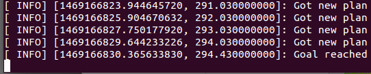
(3) mark a point coord
Next, select “Publish Point” and hover over your map (but don’t click) where you’d like TurtleBot to go when you run your script. On the bottom left corner of the screen next to “select this point” you’ll notice three numbers which change when you move the mouse. This is your point, so write these numbers down.
TIP: The third number is altitude. It may show a number that isn’t perfectly 0, but regardless of what it says, use 0.

In a new terminal window run:
$ gedit ~/helloworld/go_to_specific_point_on_map.py
Look for this line of code (line 83):
position = {‘x’: 1.22, ‘y’ : 2.56}
Overwrite the x, y values with the numbers you wrote down earlier when doing “publish point”. for eample 0.3 2.0, Save and exit.

Then run:
$ python ~/helloworld/go_to_specific_point_on_map.py

16- also, goto amazon to setup AWS with LAMP@ubuntu1404 to test browser and app.

在hydro版本的ROS，对于turtlebot机器人，只支持stage模拟器，栈和包是turtlebot_gazebo。

0、准备

0.1、如果需要，安装：
$ sudo apt-get install ros-hydro-turtlebot-simulator
0.2、如果需要，更新：
$ rosdep update
0.3、如果需要安装键盘控制
$ sudo apt-get install ros-hydro-turtlebot-apps ros-hydro-turtlebot-rviz-launchers

一、仿真：gazebo模拟world，rviz可视化。

1.1、启动gazebo模拟器下的机器人，和空的world。
$ roslaunch turtlebot_gazebo turtlebot_empty_world.launch
1.2、启动键盘控制终端，这样可以通过键盘控制机器人动作。
$ roslaunch turtlebot_teleop keyboard_teleop.launch
1.3、启动可视化窗口，这样可以显示机器人所探测的世界。
$ roslaunch turtlebot_rviz_launchers view_robot.launch
1.4.1、可以在gazebo里面放置一些障碍物，例如圆柱垃圾桶和矩形桌子

1.4.2、通过rviz，可以显示点云图

二、建图导航：进一步的建图和导航功能。

1.1、启动gazebo模拟器下的机器人和虚拟world
$ roslaunch turtlebot_gazebo turtlebot_playground.launch
1.2、启动建图
$ roslaunch turtlebot_gazebo gmapping_demo.launch
1.3、通过可视化查看建图过程
$ roslaunch turtlebot_rviz_launchers view_navigation.launch
1.4、启动键盘控制终端移动，直到地图满意为止
$ roslaunch turtlebot_teleop keyboard_teleop.launch
1.5、保存地图
$ rosrun map_server map_saver -f ~/demomap
1.6、使用地图导航：关闭所有进程，重复以上所有步骤，除了建图这一步。
$ roslaunch turtlebot_gazebo amcl_demo.launch map_file:=~/demomap.yaml

• 1、启动机器人

物理环境就是把真是机器人bring-up，这里在3d版模拟器gazebo中启动机器人turtlebot：
$ roslaunch turtlebot_gazebo turtlebot_world.launch
先启动这个gazeb就相当于把硬件启动了，传感器也都启动了，激光器/scan和里程计/odom都有数据了。
如下图这是个简单的宾馆场景：

问题一、出现Error [SDF.cc:788] Missing element description for [pointCloudCutoffMax]
解释：没找到答案。好像不会影响使用。
问题二、出现modeldatabase：unable to get model name
解释一：这是gazebo2.2太老，需要更新：
$ sudo sh -c ‘echo “deb http://packages.osrfoundation.org/gazebo/ubuntu trusty main” > /etc/apt/sources.list.d/gazebo-latest.list’
$ wget http://packages.osrfoundation.org/gazebo.key -O – | sudo apt-key add –
$ wget http://gazebosim.org/models/dumpster/model.tar.gz
解释二：这是因为它到http://gazebosim.org/models去采集组建但某种原因出现了问题，所以不如直接全部下载，几个小时。
$ cd ~/.gazebo
$ wget -r -R “index.html*” http://models.gazebosim.org/
把下载得到的都复制到~/.gazebo/models文件夹。
问题三、启动gazebo出错不能启动
解释：这通常是非nvida显卡引起的，没有办法，多启动几次总会好。

• 2、控制机器人移动

如果通过键盘
$ roslaunch turtlebot_teleop keyboard_teleop.launch –screen
如果通过罗技手柄
$ roslaunch turtlebot_teleop logitech.launch –screen

3、查看机器人

$ roslaunch turtlebot_rviz_launchers view_robot.launch
很好，机器人看起来不错。

4、创建地图

$ roslaunch turtlebot_gazebo gmapping_demo.launch
启动gmapping，就可以利用采集所得到的传感器数据，进行地图绘制，/map也就有数据了。
这个过程是静寂的。
说明一、这个terminal停留在Registering First Scan不动，这是因为机器人没有移动的缘故。
此时可以尝试调试工具：
$ rosrun rqt_graph rqt_graph
WARNING: topic [/base_scan] does not appear to be published yet

5、显示地图

Gazebo模拟了现实世界，RViz可视化的感知周围事物。所以运行rviz，显示相应的制图信息。
$ roslaunch turtlebot_rviz_launchers view_navigation.launch –screen
此时可以尝试调试工具：
$ rostopic echo /base_scan
$ rostopic echo /odom
$ rostopic echo /map | grep frame_id
$ roswtf
$ Loaded plugin tf.tfwtf No package or stack in context
根据激光扫描器安装与否，有时会把scan重定向到base_scan，这样：
$ rosrun gmapping slam_gmapping scan:=base_scan

6、移动扫描

此时控制turtle平面走动，并转圈扫描，不断丰富地图，如下图：

• 7、保存地图

如果满意，把地图保存用于后续的导航：
$ rosrun map_server map_saver -f dehaoZ_map

8、建图结束

地图构建完成后，关闭以上所有进程。看机器人如何自主导航。

$ roslaunch turtlebot_gazebo turtlebot_world.launch

$ roslaunch turtlebot_teleop keyboard_teleop.launch –screen

$ roslaunch turtlebot_gazebo amcl_demo.launch map_file:=/home/dehaoz/dehaoZ_map.yaml
这个过程也是静寂的。

$ roslaunch turtlebot_rviz_launchers view_navigation.launch

随便点击，作为目标地。规划路径及行走过程如下图：

amcl的terminal里也会提示到达目的地：

9、琐碎的事情

问题一、
rviz出错：Map “No transform from [map] to [base_link]”
解释：
You will need a transform from the /map frame to /base_link. However, there only needs to be a path between /map and /base_link, not a direct transform. Usually, the transform setup looks something like /map->/odom->/base_link.
These transforms are usually provided by a localization node such as amcl or a SLAM node such as gmapping.

问题二、
rviz出错：global status error Fixed Frame [map] does not exist
解释一、
I may not be considering this correctly, but it may be as simple as changing your “fixed frame” under “.Global Options” to “/”, “/world”, or some
fixed frame that you do have a transform for. “/base_link”！！！！
解释二、
1-这个fix frame可以解决I don’t even know how to change it. I tried your solution, it fixes “Global Status” but there still is RobotModel error:
Screenshot rosrun tf static_transform_publisher 0.0 0.0 0.0 0.0 0.0 0.0 map my_frame 100
2-You don’t have a localization as e.g. amcl running. Thus, the transformation map->base_link (or whatever you have for your robots link) does not
exist.
解释三、
You need to publish a map frame. If I’m correct, your problem is that AMCL is looking for the /map frame when it loads your static map from the map_server. In order to resolve this problem, you must either set the frame_id of your map_server to /odom or publish the /map frame as a parent
frame to /odom.

问题三、
amcl出现Extrapolation Error looking up robot pose: Lookup would require extrapolation into the past. Requested time 560.090000000 but the earliest
data is at time 620.530000000, when looking up transform from frame [base_footprint] to frame [map]
解释一、
The error is telling you that your asking for a transform from a time before which you have tf data。Most tf datasources report data in monotonic
increasing order which means that no matter long you wait you will not receive older data.。You will either need to initialize the transform listener
earlier and allow the buffer to fill up, or pass a few of these errors on startup. It’s a common race condition whether the data or tf data arrives
first.。try increasing ros::Duration(0.2) upto maximum of 10 seconds。就是说要增加延时，或者采用阻塞模式：
try{
ros::Time now = ros::Time::now();
listener.waitForTransform(“/turtle2”, “/turtle1”,now, ros::Duration(3.0));
listener.lookupTransform(“/turtle2”, “/turtle1”, now, transform);
//Note: Using ros::Time::now() is for demo， usually would be timestamp of data wishing to be transformed.
这里面waitForTransform()将会阻塞一直到坐标转换可用为止或者超时为止。
诊断二、
warn:could not get robot pose
（1）先看看大致结构。
$ rosrun rqt_graph rqt_graph
（2）再看看tf信息
$ rosrun tf tf_monitor
（3）可能会有
published by unknown_publisher
（4）看看amcl
$ rostopic info amcl_pose
（5）可以尝试
$ rosrun tf tf_echo odom map
（6）尝试减小地图尺寸
reducing size of local cost map to original size of 6×6 @ 0.5 resolution, the extrapolatoin error went away.
（7）注意CPU负载
$ gnome-system-monitor
To make sure the CPU didn’t stall, I essentially lowered the local/global maps and move_base controller update frequency to a point where the
navigation wouldn’t work well at all. For me, the map updating/publishing rates were down to 3Hz and 2Hz, respectively. The move_base frequency was
also down to 3-4Hz. On top of this, I was running rviz on the same laptop on an integrated graphics card.
1-The local planar detected an obstacle. As it moves around it, the obstacle was dragged across the local map, enclosing the robot an completely
unmovable space.
2-This lead to the robot getting lost, a lot. I would see it moving to the goal designated, but when it gets there, it would spin to get the correct
orientation. While this happens, the laser scan would slowly move out of place of the global map.Here is a couple general rule of thumb if you want
to run the navstack：Don’t run the map/controller frequency lower than the ros nav stack guide.I upgraded to a laptop with an i7-4th gen (~2.2Ghz),
and an nvidia graphics card. I run the map publish rates and controller publish rates to twice the ros tutorial’s values. It can run at higher
velocities and smoother motions!Naturally, those errors went away after the upgrade and the CPU stopped stalling/running so slow.
解释三、
是真实导航但可能使用了模拟位置：
The problem is your fake_localization. It publishes map->odom, which is now done by the real localization from the MultiMapper, So you have to remove
this fake_localization.
Somewhere in your launch file there is a node named “fake_lokalization” (I guess it is just a static_transform_publisher). Just remove this one when
adding the mapper to your system.
Looking at your RVIZ-screenshot it seems a bit like the robot is not moving the way it thinks it does. (The map patches are overlayed incorrectly.)
Some ideas only:
Check if the odometry published by Gazebo is correct. (Visualize TF in RVIZ)
Look at the Operators costmap in RVIZ (type “map”, topic “/Operator/local_costmap”)
Try to run tutorial 1 with your setup first and see if it works correctly. Then add Mapper and Navigator step by step.