按类别存档： 机器视觉

循环神经网络RNN出现于在20世纪80年代，最近由于计算能力提升得以流行起来。

RNN的网络对序列数据特别有用，因为RNN的每个神经单元能用其内部存储来保存之前输入的相关信息。注意到这点很重要，例如当阅读一个句子时，就需要从它之前的单词中提出每个词的语境。例如在语言案例中，「I had washed my house」这句话的意思与「I had my house washed」大不相同。这就能让网络获取对该表达更深的理解。
RNN的循环可以处理不定长的输入，得到一定的输出。因此当输入可长可短时， 例如训练翻译模型，其句子长度军不固定，这就无法像一个训练固定像素的图像那样用CNN搞定。

所以，善于处理序列化数据的RNN，与，善于处理图像等静态类变量的CNN相比，最大区别就是循环这个核心特征，即系统的输出会保留在网络里和系统下一刻的输入一起共同决定下一刻的输出，即此刻的状态包含上一刻的历史，又是下一刻变化的依据。

1. RNN 温习
收起的循环神经网络是这样，内部有个闭环:

展开的循环神经网络是这样，在时间轴上：

上图中， xt是某些输入，A是循环神经网络的一部分，ht是t时刻输出。

或者，换句话说，隐藏层的反馈，不仅仅进入了输出端，还还进入到了下一时间的隐藏层。

前面是一个单元的， 两个单元的情况是这样：
收起的：

以上的网络可以通过两个时间步来展开，将连接以无环的形式可视化：

这样递归网络有时被描述为深度网络，其深度不仅仅发生在输入和输出之间，而且还发生在跨时间步，每个时间步可以被认为是一个层；不过，权重（从输入到隐藏和隐藏到输出）在每个时间步是相同的。

1.1 前向传播

将网络按时间展开是这样：

则其前向传播：

其中：
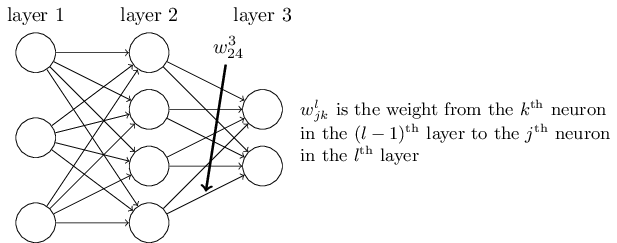
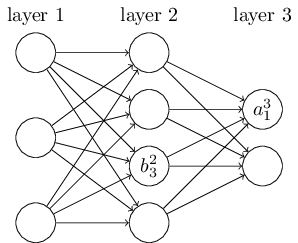
下标， i表示输入层 ， h为隐藏层 ，k为输出层。
参数， a表示未激活值， b表示激活值。
REF： http://www.voidcn.com/blog/dream_catcher_10/article/p-2421992.html

1.3 反向传播

训练RNN和训练传统神经网络相似，同样要使用反向传播算法，但会有一些变化。因为参数在网络的所有时刻是共享的，每一次的梯度输出不仅依赖于当前时刻的计算结果，也依赖于之前所有时刻的计算结果。

例如，为了计算时刻t=4的梯度，需要反向传播3步，并把前面的所有梯度加和。这被称作随时间的反向传播（BPTT）。只要知道普通的用BPTT训练的RNN对于学习长期依赖（相距很长时间的依赖）是很困难的，因为这里存在梯度消失或爆炸问题。当然也存在一些机制来解决这些问题，特定类型的RNN（如LSTM）就是专门设计来解决这些问题的。

1.5 LSTM扩展

这些年来，研究者已经提出了更加复杂的RNN类型来克服普通RNN模型的缺点。例如Bidirectional 和LSMT。
Bidirectional RNN的思想是时刻的输出不仅依赖于序列中之前的元素，也依赖于之后的元素。例如，要预测一句话中缺失的词，可能需要左右上下文。Bidirecrtional RNN很直观，只是两个RNN相互堆叠在一起，输出是由两个RNN的隐藏状态计算得到的。

LSTM network最近非常流行，上面也简单讨论过。LSTM与RNN在结构上并没有本质的不同，只是使用了不同的函数来计算隐藏状态。LSTM中的记忆单元被称为细胞，可以把它当作是黑盒，它把前一刻的状态ht-1和当前输入xt。内部这些细胞能确定什么被保存在记忆中，什么被从记忆中删除。
这些细胞把之前的状态，当前的记忆和输入结合了起来，事实证明这些类型的单元对捕捉长期依赖十分有效。LSTM在刚开始时会让人觉得困惑。
理论上说，循环神经网络能从句子开头处理语境，它允许对一个句子末尾的词进行更精确的预测。
在实践中，对于 vanilla RNN， 也就是传统的卷积网络 cnn， 来说，这并不是真正需要的。这就是为什么 RNN 在出现之后淡出研究圈一段时间直到使用神经网络中的长短期记忆（LSTM）单元取得了一些不错的结果后又重新火起来的主要原因。

加上 LSTM 后的网络就像是加了一个记忆单元，能记住输入的最初内容的语境。

这些少量记忆单元能让 RNN 更加精确，而且是这种模型流行的最新原因。
这些记忆单元允许跨输入以便记住上下文语境。这些单元中，LSTM 与门控循环单元（GRU）是当下使用比较广泛的两个，后者的计算效率更高，因为它们占用的计算机内存比较少。

3. RNN 典型应用

3.1 文学创作

RNN 有很多应用，其中一个不错的应用是自然语言处理NLP，已经有很多人验证了 RNN创造出令人惊讶的模型，这些模型能表示一种语言模型。
这些语言模型能采纳像莎士比亚的诗歌这样的大量输入，并在训练这些模型后生成它们自己的莎士比亚式的诗歌，而且这些诗歌很难与原作区分开来。

REF : http://www.jiqizhixin.com/article/1410

这种特殊类型的 RNN 是在一个文本数据集中喂养的，它要逐字读取输入。
与一次投喂一个词相比，这种方式让人惊讶的地方是这个网络能创造出它自己独特的词，这些词是用于训练的词汇中没有的。

这张从以上参考文章中摘取的图表展示了这个 char RNN 模型将会如何预测「Hello」这个词。这张图很好地将网络如何逐字采纳每个词并预测下一个字符的可能性可视化了。

3.3 机器翻译

这种方法很有趣，因为它需要同时训练两个 RNN。
在这些网络中，输入的是成对的不同语言的句子。例如，给这个网络输入意思相同的一对英法两种语言的句子，其中英语是源语言，法语作为翻译语言。有了足够的训练后，给这个网络一个英语句子，它就能把它翻译成法语.

这模型被称为序列到序列模型（Sequence to Sequences model ）或者编码器-解码器模型（Encoder- Decoder model）。

英法翻译的例子

这张图表展示了信息流是如何通过编码-解码模型的，它用了一个词嵌入层（ word embedding layer ）来获取更好的词表征。
一个词嵌入层通常是 GloVe 或者 Word 2 Vec 算法，能批量采纳词，并创建一个权重矩阵，让相似的词相互连接起来。
用一个嵌入层通常会让 RNN 更加精确，因为它能更好的表征相似的词是什么样的，以便减少网络的推断。

3.5 图片描述

We present a model that generates natural language descriptions of images and their regions. Our approach leverages datasets of images and their sentence descriptions to learn about the inter-modal correspondences between language and visual data. Our alignment model is based on a novel combination of Convolutional Neural Networks over image regions, bidirectional Recurrent Neural Networks over sentences, and a structured objective that aligns the two modalities through a multimodal embedding. We then describe a Multimodal Recurrent Neural Network architecture that uses the inferred alignments to learn to generate novel descriptions of image regions
We demonstrate that our alignment model produces state of the art results in retrieval experiments on Flickr8K, Flickr30K and MSCOCO datasets. We then show that the generated descriptions significantly outperform retrieval baselines on both full images and on a new dataset of region-level annotations. Under NVIDIA Corporation the GPUs.

图面描述，很好。

视觉语义排列，不错。

REF： http://cs.stanford.edu/people/karpathy/deepimagesent/
code： https://github.com/karpathy/neuraltalk

5. RNN的字符级语言模型 – Char RNNs – character level language model

具体的，RNN用于语言处理NLP时， 能输入句子中的单词，或者，单词中的字符，然后通过该循环神经网络它会得出。
对于下图的RNN模型的架构：

隐藏层都有多个神经元，单独的每个神经元的输入和输出情况是这样：

网络结构的含义：
各个垂直矩形框，代表每轮迭代的隐藏层；
xt，是隐层的输入，而且隐层将产生两个，一个预测输出值y^，一个提供给下一层隐层的输出特征向量ht。

网络中各个参数的含义：
x1,…,xt−1,xt,xt+1,…,xT， 表示拥有T个数量词汇的语料中，各个词汇对应的词向量。
ht， 表示每一轮迭代t中，用于计算隐藏层的输出特征的传递边。
ht-1， 在前一轮迭代t−1中，非线性函数的输出结果。
Whx， 输入层x到隐藏层h的， 利用输入词xt作为条件，计算得到的， 权重矩阵。
Whh， 隐藏层h到隐藏层h的， 利用前一轮迭代的输出作为条件， 计算得到的， 权重矩阵。
σ()， 非线性分类函数，例如使用sigmoid分类函数。
y^t， 每一轮迭代t，针对全部词汇的输出概率分布。

REF： http://blog.csdn.net/han_xiaoyang/article/details/51932536

其后的目标是说明基于循环网络RNN的一个字符级的语言模型所能完成的任务。有两个方面的应用：
一，基于每个序列在现实世界中出现的可能性对其进行打分，这实际上提供了一个针对语法和语义正确性的度量，语言模型通常为作为机器翻译系统的一部分。
二，语言模型可以用来生成新文本。根据莎士比亚的作品训练语言模型可以生成莎士比亚风格的文本。
REF : http://karpathy.github.io/2015/05/21/rnn-effectiveness/ <— 梯子
Code ： https://github.com/karpathy/char-rnn

There’s something magical about Recurrent Neural Networks (RNNs).
Sometimes the ratio of how simple your model is to the quality of the results you get out of it blows past your expectations, and this was one of those times. What made this result so shocking at the time was that the common wisdom was that RNNs were supposed to be difficult to train (with more experience I’ve in fact reached the opposite conclusion).
By the way, code on Github that allows you to train character-level language models based on multi-layer LSTMs. You give it a large chunk of text and it will learn to generate text like it one character at a time. You can also use it to reproduce my experiments below.

1. 什么是 RNN

1.1 序列情况 – Sequences

A glaring limitation of Vanilla Neural Networks (and also Convolutional Networks) ， is that their API is too constrained: they accept a fixed-sized vector as input (e.g. an image) ， and produce a fixed-sized vector as output (e.g. probabilities of different classes).

Not only that: These models perform this mapping using a fixed amount of computational steps (e.g. the number of layers in the model). The core reason that recurrent nets are more exciting is that they allow us to operate over sequences of vectors: Sequences in the input, the output, or in the most general case both.

RNN的几个应用场景 – A few examples may make this more concrete:

Each rectangle is a vector， and， arrows represent functions (e.g. matrix multiply).
Input vectors are in red, output vectors are in blue， and green vectors hold the RNN’s state (more on this soon).
From left to right:
(1) Vanilla mode of processing without RNN, from fixed-sized input to fixed-sized output (e.g. image classification).
(2) Sequence output (e.g. image captioning， takes an image and outputs a sentence of words).
(3) Sequence input (e.g. sentiment analysis， where a given sentence is classified as expressing positive or negative sentiment).
(4) Sequence input and sequence output (e.g. Machine Translation， an RNN reads a sentence in English and then outputs a sentence in French).
(5) Synced sequence input and output (e.g. video classification， where we wish to label each frame of the video).
Notice that in every case are no pre-specified constraints on the lengths sequences because the recurrent transformation (green) is fixed and can be applied as many times as we like.

As you might expect, the sequence regime of operation is much more powerful compared to fixed networks that are doomed from the get-go by a fixed number of computational steps, and hence also much more appealing for those of us who aspire to build more intelligent systems.

Moreover, as we’ll see in a bit, RNNs combine the input vector with their state vector with a fixed (but learned) function to produce a new state vector. This can in programming terms be interpreted as running a fixed program with certain inputs and some internal variables.

Viewed this way, RNNs essentially describe programs. In fact, it is known that RNNs are Turing-Complete in the sense that they can to simulate arbitrary programs (with proper weights). But similar to universal approximation theorems for neural nets you shouldn’t read too much into this. In fact, forget I said anything. see：

CNN和RNN的区别：If training vanilla neural nets is optimization over functions, training recurrent nets is optimization over programs.
REF http://binds.cs.umass.edu/papers/1995_Siegelmann_Science.pdf

1.3 非序列场景 – Sequential processing in absence of sequences

You might be thinking that having sequences as inputs or outputs could be relatively rare, but an important point to realize is that even if your inputs/outputs are fixed vectors, it is still possible to use this powerful formalism to process them in a sequential manner.

For instance, the figure below shows results from two very nice papers from DeepMind.
On the left, an algorithm learns a recurrent network policy that steers its attention around an image; In particular, it learns to read out house numbers from left to right (Ba et al.).
On the right, a recurrent network generates images of digits by learning to sequentially add color to a canvas (Gregor et al.) 。

Left: RNN learns to read house numbers. Right: RNN learns to paint house numbers.

The takeaway is that even if your data is not in form of sequences, you can still formulate and train powerful models that learn to process it sequentially. You’re learning stateful programs that process your fixed-sized data.

1.5 RNN computation

So how do these things work?
At the core, RNNs have a deceptively simple API: They accept an input vector x and give you an output vector y.
However, crucially this output vector’s contents are influenced not only by the input you just fed in, but also on the entire history of inputs you’ve fed in in the past. 然而这个输出向量的内容不仅被输入数据影响，而且会收到整个历史输入的影响。写成一个类的话，RNN的API只包含了一个step方法：
rnn = RNN()
y = rnn.step(x) # x is an input vector, y is the RNN’s output vector

每当step方法被调用的时候，RNN的内部状态就被更新。在最简单情况下，该内部装着仅包含一个简单的内部隐向量hh。
下面是一个普通RNN的step方法的实现
class RNN:
# …
def step(self, x):
# update the hidden state
self.h = np.tanh(np.dot(self.W_hh, self.h) + np.dot(self.W_xh, x))
# compute the output vector
y = np.dot(self.W_hy, self.h)
return y
以上就是RNN的前向传输 – The above specifies the forward pass of a vanilla RNN.

参数：
h是hidden variable 隐变量，即整个网络每个神经元的状态。 这个隐藏状态self.h被初始化为零向量。
x是输入，
y是输出，
h，x，y 三者都是高维向量。
RNN的参数是三个矩阵 W_hh, W_xh, W_hy。 – This RNN’s parameters are the three matrices W_hh, W_xh, W_hy.
np.tanh函数是一个非线性函数，可以将激活数据挤压到[-1,1]之内。

隐变量 h，就是通常说的神经网络本体，也正是循环得以实现的基础， 因为它如同一个可以储存无穷历史信息(理论上)的水库，一方面会通过输入矩阵W_xh吸收输入序列x的当前值，一方面通过网络连接W_hh进行内部神经元间的相互作用（网络效应，信息传递），因为其网络的状态也和输入的整个过去历史有关， 最终的输出是两部分加在一起共同通过非线性函数tanh。整个过程就是一个循环神经网络“循环”的过程。
参数 W_hh理论上可以可以刻画输入的整个历史对于最终输出的任何反馈形式，从而刻画序列内部，或序列之间的时间关联， 这是RNN之所以强大的关键。

关于代码：
在tanh内有两个部分。一个是基于前一个隐藏状态，另一个是基于当前的输入。
在numpy中，np.dot是进行矩阵乘法。先两个中间变量相加，其结果被tanh处理为一个新的状态向量。

联想：
RNN本质是一个数据推断（inference）机器， 只要数据足够多，就可以得到从x（t）到y（t）的概率分布函数， 寻找到两个时间序列之间的关联，从而达到推断和预测的目的。
这会让人联想到另一个时间序列推断的隐马尔科夫模型 HMM， 在HM模型里同样也有一个输入x和输出y和一个隐变量h。
而HMM这个h， 和， RNN里的h， 区别在于迭代法则： HMM通过跃迁矩阵把此刻的h和下一刻的h联系在一起，跃迁矩阵随时间变化；而RNN中没有跃迁矩阵的概念，取而代之的是神经元之间的连接矩阵。 此外， HMM本质是一个贝叶斯网络， 因此每个节点都是有实际含义的； 而RNN中的神经元只是信息流动的枢纽而已，并无实际对应含义。但是， HMM能干的活， RNN几乎也是可以做的，比如语言模型，就是RNN的维度会更高一些。

1.7 更深层网络 – Going deep

RNNs are neural networks and everything works monotonically better (if done right) if you put on your deep learning hat and start stacking models up like pancakes. RNN属于神经网络算法，如果你像叠薄饼一样开始对模型进行重叠来进行深度学习，那么算法的性能会单调上升（如果没出岔子的话）。

For instance, we can form a 2-layer recurrent network as follows:
y1 = rnn1.step(x)
y = rnn2.step(y1)

Except neither of these RNNs know or care – it’s all just vectors coming in and going out, and some gradients flowing through each module during backpropagation. 它们并不在乎谁是谁的输入：都是向量的进进出出，都是在反向传播时梯度通过每个模型。

1.9 LSTM – Getting fancy

I’d like to briefly mention that in practice most of us use a slightly different formulation than what I presented above called a Long Short-Term Memory (LSTM) network.

The LSTM is a particular type of recurrent network that works slightly better in practice, owing to its more powerful update equation and some appealing backpropagation dynamics. I won’t go into details, but everything I’ve said about RNNs stays exactly the same, except the mathematical form for computing the update (the line self.h = … ) gets a little more complicated.

From here on I will use the terms “RNN/LSTM” interchangeably but all experiments in this post use an LSTM.

更好的网络。需要简要指明的是在实践中通常使用的是一个稍有不同的算法，长短基记忆网络，简称LSTM。
LSTM是循环网络的一种特别类型。由于其更加强大的更新方程和更好的动态反向传播机制，它在实践中效果要更好一些。
本文不会进行细节介绍，但是在该算法中，所有介绍的关于RNN的内容都不会改变，唯一改变的是状态更新（就是self.h=…那行代码）变得更加复杂。
从这里开始会将术语RNN和LSTM混合使用，但是在本文中的所有实验都是用LSTM完成的。

3. 字符级语言模型 – Character Level Language Models

目标是训练一个RNN，在字符集h-e-lo中，给输入hell，可以得输出ello，即预测单词hello。

3.1 process

We’ll now ground this in a fun application: We’ll train RNN character-level language models. That is, we’ll give the RNN a huge chunk of text and ask it to model the probability distribution of the next character in the sequence given a sequence of previous characters. This will then allow us to generate new text one character at a time.

As a working example, suppose we only had a vocabulary of four possible letters h-e-l-o, and wanted to train an RNN on the training sequence “hello”. This training sequence is in fact a source of 4 separate training examples:
1. The probability of “e” should be likely given the context of “h”,
2. “l” should be likely in the context of “he”,
3. “l” should also be likely given the context of “hel”,
4. and finally “o” should be likely given the context of “hell”.

3.3 one hot encoding

One hot encoding，transforms categorical features to a format that works better with classification and regression algorithms.
Let’s take the following example. I have seven sample inputs of categorical data belonging to four categories.
Now, I could encode these to nominal values as I have done here, but that wouldn’t make sense from a machine learning perspective.
We can’t say that the category of “Penguin” is greater or smaller than “Human”. Then they would be ordinal values, not nominal.

What we do instead is generate one boolean column for each category.
Only one of these columns could take on the value 1 for each sample. Hence, the term one hot encoding.

This works very well with most machine learning algorithms.

3.5 detailed process

Concretely, we will encode each character into a vector using 1-of-k encoding (i.e. all zero except for a single one at the index of the character in the vocabulary), and feed them into the RNN one at a time with the step function.
We will then observe a sequence of 4-dimensional output vectors (one dimension per character), which we interpret as the confidence the RNN currently assigns to each character coming next in the sequence.
Here’s a diagram:

An example RNN with 4-dimensional input and output layers, and a hidden layer of 3 units (neurons). This diagram shows the activations in the forward pass when the RNN is fed the characters “hell” as input. The output layer contains confidences the RNN assigns for the next character (vocabulary is “h,e,l,o”); We want the green numbers to be high and red numbers to be low.

For example, we see that in the first time step when the RNN saw the character “h” it assigned confidence of 1.0 to the next letter being “h”, 2.2 to letter “e”, -3.0 to “l”, and 4.1 to “o”.
Since in our training data (the string “hello”) the next correct character is “e”, we would like to increase its confidence (green) and decrease the confidence of all other letters (red).
Similarly, we have a desired target character at every one of the 4 time steps that we’d like the network to assign a greater confidence to.
Since the RNN consists entirely of differentiable operations we can run the backpropagation algorithm (this is just a recursive application of the chain rule from calculus) to figure out in what direction we should adjust every one of its weights to increase the scores of the correct targets (green bold numbers).
We can then perform a parameter update, which nudges every weight a tiny amount in this gradient direction.
If we were to feed the same inputs to the RNN after the parameter update we would find that the scores of the correct characters (e.g. “e” in the first time step) would be slightly higher (e.g. 2.3 instead of 2.2), and the scores of incorrect characters would be slightly lower.
We then repeat this process over and over many times until the network converges and its predictions are eventually consistent with the training data in that correct characters are always predicted next.

A more technical explanation is that we use the standard Softmax <<<>>> classifier (also commonly referred to as the cross-entropy loss) on every output vector simultaneously.
The RNN is trained with mini-batch Stochastic Gradient Descent and I like to use RMSProp or Adam (per-parameter adaptive learning rate methods) to stablilize the updates.

Notice also that the first time the character “l” is input, the target is “l”, but the second time the target is “o”.
The RNN therefore cannot rely on the input alone and must use its recurrent connection to keep track of the context to achieve this task.
是的。

At test time, we feed a character into the RNN and get a distribution over what characters are likely to come next. We sample from this distribution, and feed it right back in to get the next letter. Repeat this process and you’re sampling text!
Lets now train an RNN on different datasets and see what happens.

To further clarify, for educational purposes I also wrote a minimal character-level RNN language model in Python/numpy. It is only about 100 lines long and hopefully it gives a concise, concrete and useful summary of the above if you’re better at reading code than text. We’ll now dive into example results, produced with the much more efficient Lua/Torch codebase.

5. Python 的代码实现

可以直接进入character-level RNN， PhD Karpathy用Python写了一个 RNN语言模型的Demo， 只有100行代码。
REF ： http://jaybeka.github.io/2016/05/18/rnn-intuition-practice/
code: https://gist.github.com/karpathy/d4dee566867f8291f086
现在Karpathy及其团队已经专注于更快更强的Lua/Torch代码库。

“””
Minimal character-level Vanilla RNN model. Written by Andrej Karpathy (@karpathy)
BSD License
“””
import numpy as np

## 导入纯文本文件，建立词到索引和索引到词的两个映射
data = open(‘input.txt’, ‘r’).read() # 读整个文件内容，得字符串str类型data
chars = list(set(data)) # 去除重复的字符，获得不重复字符
data_size, vocab_size = len(data), len(chars) # 源文件的字符总数和去除重复后的字符数
print ‘data has %d characters and %d unique.’ % (data_size, vocab_size)
char_to_ix = { ch:i for i,ch in enumerate(chars) }
ix_to_char = { i:ch for i,ch in enumerate(chars) }
# 用enumerate函数把字符表达成向量，如同构建语言的数字化词典
# 这一步后，语言信息就变成了数字化的时间序列

## hyperparameters
## 定义隐藏层神经元数量，每一步处理序列的长度，以及学*速率
hidden_size = 100 # 隐藏层神经元个数
seq_length = 25 # number of steps to unroll the RNN for
learning_rate = 1e-1 # 学*率

## model parameters
## 随机生成神经网络参数矩阵，Wxh即U，Whh即W，Why即V，以及偏置单元
Wxh = np.random.randn(hidden_size, vocab_size)*0.01 # input to hidden
Whh = np.random.randn(hidden_size, hidden_size)*0.01 # hidden to hidden
Why = np.random.randn(vocab_size, hidden_size)*0.01 # 隐藏层到输出层，输出层预测的是每个字符的概率
bh = np.zeros((hidden_size, 1)) # hidden bias 隐藏层偏置项
by = np.zeros((vocab_size, 1)) # output bias 输出层偏置项
# 上面初始化三个矩阵W_xh， W_hh，W_hy
# 分别是输入和隐层， 隐层和隐层， 隐层和输出，之间的连接
# 同时初始化隐层和输出层的激活函数中的bias，bh和by

## loss function 这个函数的输出是错误的梯度

def lossFun(inputs, targets, hprev):
“””
inputs,targets are both list of integers.
inputs t时刻序列，相当于输入, targets t+1时刻序列，相当于输入
hprev is Hx1 array of initial hidden state
hprev t-1时刻的，隐藏层神经元的激活值
returns the loss, gradients on model parameters, and last hidden state
“””
xs, hs, ys, ps = {}, {}, {}, {} # ps是归一化的概率
hs[-1] = np.copy(hprev) # hprev 中间层的值, 存作-1，为第一个做准备
loss = 0

## forward pass ：
## 正向传播过程，输入采用1-k向量表示，隐藏层函数采用tanh
for t in xrange(len(inputs)): # 不像range（）返回列表，xrange（）返回的对象效率更高
# 把输入编码成0-1格式,在input中,0代表此字符未激活
xs[t] = np.zeros((vocab_size,1)) # encode in 1-of-k representation
xs[t][inputs[t]] = 1 # x[t] 是一个第t个输入单词的向量
# RNN的隐藏层神经元激活值计算
# 双曲正切, 激活函数, 作用类似sigmoid
# hidden state 参考文献Learning Recurrent Neural Networks with Hessian-Free Optimization
# 生成新的中间层
hs[t] = np.tanh(np.dot(Wxh, xs[t]) + np.dot(Whh, hs[t-1]) + bh)
# RNN的输出
ys[t] = np.dot(Why, hs[t]) + by # unnormalized log probabilities for next chars
# 概率归一化
ps[t] = np.exp(ys[t]) / np.sum(np.exp(ys[t])) # probabilities for next chars
# 预期输出是1，因此这里的value值就是此次的代价函数，
# 使用 -log(*) 使得离正确输出越远，代价函数就越高
# softmax 损失函数
loss += -np.log(ps[t][targets[t],0]) # softmax (cross-entropy loss)

## backward pass: compute gradients going backwards
# 将输入循环一遍以后，得到各个时间段的h, y 和 p
# 得到此时累积的loss, 准备进行更新矩阵
dWxh, dWhh, dWhy = np.zeros_like(Wxh), np.zeros_like(Whh), np.zeros_like(Why) # 各矩阵的参数进行
dbh, dby = np.zeros_like(bh), np.zeros_like(by)
dhnext = np.zeros_like(hs[0]) # 下一个时间段的潜在层，初始化为零向量
for t in reversed(xrange(len(inputs))): # 把时间作为维度，则梯度的计算应该沿着时间回溯
dy = np.copy(ps[t]) # 设dy为实际输出，而期望输出（单位向量）为y, 代价函数为交叉熵函数
dy[targets[t]] -= 1 # backprop into y.
# see cs231n.github.io/neural-networks-case-study
# grad if confused here
dWhy += np.dot(dy, hs[t].T) # dy * h(t).T， h层值越大的项，如果错误，则惩罚越严重。
# 反之，奖励越多（这边似乎没有考虑softmax的求导？）
dby += dy # 这个没什么可说的，与dWhy一样，
# 只不过h项=1， 所以直接等于dy
dh = np.dot(Why.T, dy) + dhnext # backprop into h 第一阶段求导
dhraw = (1 – hs[t] * hs[t]) * dh # backprop through tanh nonlinearity #第二阶段求导，注意tanh的求导
dbh += dhraw # dbh表示传递 到h层的误差
dWxh += np.dot(dhraw, xs[t].T) # 对Wxh的修正，同Why
dWhh += np.dot(dhraw, hs[t-1].T) # 对Whh的修正
dhnext = np.dot(Whh.T, dhraw) # h层的误差通过Whh不停地累积
for dparam in [dWxh, dWhh, dWhy, dbh, dby]:
np.clip(dparam, -5, 5, out=dparam) # clip to mitigate exploding gradients
return loss, dWxh, dWhh, dWhy, dbh, dby, hs[len(inputs)-1]

## 预测函数，用于验证
## 给定seed_ix为t=0时刻的字符索引，生成预测后面的n个字符
## 这个sample函数就是给一个首字母，然后神经网络会输出下一个字母
def sample(h, seed_ix, n):
“””
sample a sequence of integers from the model
h is memory state, seed_ix is seed letter for first time step
“””
x = np.zeros((vocab_size, 1))
x[seed_ix] = 1
ixes = []
for t in xrange(n):
# h是递归更新的
h = np.tanh(np.dot(Wxh, x) + np.dot(Whh, h) + bh) # 更新中间层
y = np.dot(Why, h) + by # 得到输出
p = np.exp(y) / np.sum(np.exp(y)) # softmax
# 根据概率大小挑选:
# 由softmax得到的结果，按概率产生下一个字符
ix = np.random.choice(range(vocab_size), p=p.ravel())
# ravel展平数组元素的顺序通常是C风格，就是说最右边的索引变化得最快，因此元素a[0,0]之后是a[0,1]
# random.choice()从range(vocab_size)按照p=p.ravel概率随机选取默认长度1的内容放入ix
# 更新输入向量
x = np.zeros((vocab_size, 1)) # 产生下一轮的输入
x[ix] = 1
# 保存序列索引
ixes.append(ix)
return ixes

## 主程序很简单 ##

n, p = 0, 0 # n表示迭代网络迭代训练次数
mWxh, mWhh, mWhy = np.zeros_like(Wxh), np.zeros_like(Whh), np.zeros_like(Why) # 初始三个派生子矩阵
mbh, mby = np.zeros_like(bh), np.zeros_like(by) # memory variables for Adagrad
smooth_loss = -np.log(1.0/vocab_size)*seq_length # loss at iteration 0

# n表示迭代网络迭代训练次数
# 当输入是t=0时刻时，它前一时刻的隐藏层神经元的激活值我们设置为0
# while n<20000: while True: # prepare inputs (we’re sweeping from left to right in steps seq_length long) if p+seq_length+1 >= len(data) or n == 0: # 如果 n=0 或者 p过大， data是读整个文件内容得字符串str类型
hprev = np.zeros((hidden_size,1)) # reset RNN memory,中间层内容初始化,零初始化
p = 0 # go from start of data , p 重置
# 输入与输出
inputs = [char_to_ix[ch] for ch in data[p:p+seq_length]] # 一批输入seq_length个字符
targets = [char_to_ix[ch] for ch in data[p+1:p+seq_length+1]] # targets是对应的inputs的期望输出。

# sample from the model now and then
# 每循环100词， sample一次，显示结果
if n % 100 == 0:
sample_ix = sample(hprev, inputs[0], 200)
txt = ”.join(ix_to_char[ix] for ix in sample_ix)
print ‘—-n %s n—-‘ % (txt, )
# 上面做的是每训练一百步看看效果， 看RNN生成的句子是否更像人话。
# Sample的含义就是给他一个首字母，然后神经网络会输出下一个字母
# 然后这两个字母一起作为再下一个字母的输入，依次类推

# forward seq_length characters through the net and fetch gradient
# RNN前向传导与反向传播，获取梯度值

loss, dWxh, dWhh, dWhy, dbh, dby, hprev = lossFun(inputs, targets, hprev)
smooth_loss = smooth_loss * 0.999 + loss * 0.001 # 将原有的Loss与新loss结合起来
if n % 100 == 0: print ‘iter %d, loss: %f’ % (n, smooth_loss) # print progress
# 这一步是寻找梯度， loss function即计算梯度 ，
# loss function的具体内容关键即测量回传的信息以供学习。
# 函数内容在最后放出最后一步是根据梯度调整参数的值，即学习的过程。

# perform parameter update with Adagrad
# 采用Adagrad自适应梯度下降法,可参看博文
# blog.csdn.net/danieljianfeng/article/details/429****21
for param, dparam, mem in zip([Wxh, Whh, Why, bh, by],
[dWxh, dWhh, dWhy, dbh, dby],
[mWxh, mWhh, mWhy, mbh, mby]):
mem += dparam * dparam # 梯度的累加
# 自适应梯度下降公式
# adagrad update 随着迭代次数增加，参数的变更量会越来越小
param += -learning_rate * dparam / np.sqrt(mem + 1e-8) # adagrad update
p += seq_length # move data pointer 批量训练
n += 1 # iteration counter 记录迭代次数
## 上面是主程序，简单 ##

7. LSTM

LSTM（Long short term memory）顾名思义， 是增加了记忆功能的RNN。
首先为什么要给RNN增加记忆呢？ 这里就要提到一个有趣的概念叫梯度消失（Vanishing Gradient），刚刚说RNN训练的关键是梯度回传，梯度信息在时间上传播是会衰减的， 那么回传的效果好坏， 取决于这种衰减的快慢， 理论上RNN可以处理很长的信息， 但是由于衰减， 往往事与愿违， 如果要信息不衰减， 就要给神经网络加记忆，这就是LSTM的原理了。

这里首先再增加一个隐变量作为记忆单元，然后把之前一层的神经网络再增加三层， 分别是输入门，输出门，遗忘门， 这三层门就如同信息的闸门， 控制多少先前网络内的信息被保留， 多少新的信息进入，而且门的形式都是可微分的sigmoid函数，确保可以通过训练得到最佳参数。
信息闸门的原理另一个巧妙的理解是某种“惯性” 机制，隐变量的状态更新不是马上达到指定的值，而是缓慢达到这个值， 如同让过去的信息多了一层缓冲，而要多少缓冲则是由一个叫做遗忘门的东西决定的。 如此发现其实这几个新增加的东西最核心的就是信息的闸门遗忘门。 根据这一原理，可以抓住本质简化lstm，如GRU或极小GRU。 其实只需要理解这个模型就够了，而且它们甚至比lstm更快更好。

看一下最小GRU的结构：

摘自： Minimal Gated Unit for Recurrent Neural Networks
第一个方程f 即遗忘门，
第二方程如果对比先前的RNN会发现它是一样的结构，只是让遗忘门f来控制每个神经元放多少之前信息出去（改变其它神经元的状态），
第三个方程描述“惯性” ，即最终每个神经元保持多少之前的值，更新多少。
这个结构就理解了记忆体RNN的精髓。

好了是时候看一下google 翻译是怎么， 首先，翻译是沟通两个不同的语言， 而要这个沟通的本质是因为它们所表达的事物是相同的， 大脑做翻译的时候，也是根据它们所表达的概念相同比如苹果-vs-apple来沟通两个语言的。如果汉语是输入，英语是输出，神经网络事实上做的是这样一件事：
Encoding： 用一个LSTM把汉语变成神经代码
Decoding：用另一个LSTM把神经代码转化为英文。
第一个lstm的输出是第二个lstm的输入， 两个网络用大量语料训练好即可。 Google在2016加入了attention机制 ，这样google的翻译系统就更接近人脑。

运用记忆神经网络翻译的核心优势是我们可以灵活的结合语境，实现句子到句子，段落到段落的过度， 因为记忆特性使得网络可以结合不同时间尺度的信息而并非只抓住个别单词， 这就好像能够抓住语境而非只是望文生义。也是因为这个RNN有着无穷无尽的应用想象力，在google翻译以及rnn的各种应用。

9. Keras 库

优点：
文档非常全且细致。
提供较为上层的框架，搞个深度学习的原型非常方便。
更新很快，且基于Python，支持CPU、GPU运算。
现在已经可以切换backend了，可以选择用theano还是用tensorflow
缺点：
原理上理解还是建议动手去搭
运行效率较低
调试不易
更新太快，Github上面的基于Keras的代码基本要根据最新的文档改一遍才能用。

项目地址：https://github.com/fchollet/keras
文档地址：http://keras.io/

# -*- coding: utf-8 -*-
“””
Created on Sat May 21 14:34:08 2016
@author: yangsicong
“””
import numpy as np

from keras.models import Sequential
from keras.layers.core import Dense, Activation, Dropout, TimeDistributedDense
from keras.layers.recurrent import LSTM

text = open(‘./input.txt’, ‘r’).read()
char_to_idx = { ch: i for (i, ch) in enumerate(sorted(list(set(text)))) }
idx_to_char = { i: ch for (ch, i) in char_to_idx.items() }
vocab_size = len(char_to_idx)

print(‘Working on %d characters (%d unique)’ % (len(text), vocab_size))

SEQ_LENGTH = 64
BATCH_SIZE = 16
BATCH_CHARS = len(text) / BATCH_SIZE
LSTM_SIZE = 512
LAYERS = 3

def read_batches(text):
T = np.asarray([char_to_idx[c] for c in text], dtype=np.int32)
X = np.zeros((BATCH_SIZE, SEQ_LENGTH, vocab_size))
Y = np.zeros((BATCH_SIZE, SEQ_LENGTH, vocab_size))

for i in range(0, BATCH_CHARS – SEQ_LENGTH – 1, SEQ_LENGTH):
X[:] = 0
Y[:] = 0
for batch_idx in range(BATCH_SIZE):
start = batch_idx * BATCH_CHARS + i
for j in range(SEQ_LENGTH):
X[batch_idx, j, T[start+j]] = 1
Y[batch_idx, j, T[start+j+1]] = 1

yield X, Y

def build_model(batch_size, seq_len):
model = Sequential()
model.add(LSTM(LSTM_SIZE, return_sequences=True, batch_input_shape=(batch_size, seq_len, vocab_size), stateful=True))
model.add(Dropout(0.2))
for l in range(LAYERS – 1):
model.add(LSTM(LSTM_SIZE, return_sequences=True, stateful=True))
model.add(Dropout(0.2))

model.add(TimeDistributedDense(vocab_size))
model.add(Activation(‘softmax’))
model.compile(loss=’categorical_crossentropy’, optimizer=’adagrad’)
return model

print ‘Building model.’
test_model = build_model(1, 1)
training_model = build_model(BATCH_SIZE, SEQ_LENGTH)
print ‘… done’

def sample(epoch, sample_chars=256):
test_model.reset_states()
test_model.load_weights(‘./tmp/keras_char_rnn.%d.h5’ % epoch)
header = ‘LSTM based ‘
sampled = [char_to_idx[c] for c in header]

for c in header:
batch = np.zeros((1, 1, vocab_size))
batch[0, 0, char_to_idx[c]] = 1
test_model.predict_on_batch(batch)

for i in range(sample_chars):
batch = np.zeros((1, 1, vocab_size))
batch[0, 0, sampled[-1]] = 1
softmax = test_model.predict_on_batch(batch)[0].ravel()
sample = np.random.choice(range(vocab_size), p=softmax)
sampled.append(sample)

print ”.join([idx_to_char[c] for c in sampled])

for epoch in range(100):
for i, (x, y) in enumerate(read_batches(text)):
loss = training_model.train_on_batch(x, y)
print epoch, i, loss

if i % 1000 == 0:
training_model.save_weights(‘./tmp/keras_char_rnn.%d.h5’ % epoch, overwrite=True)
sample(epoch)

跑两天。。。

11. with the much more efficient Lua/Torch codebase.

All 5 example character models below were trained with the code I’m releasing on Github. The input in each case is a single file with some text, and we’re training an RNN to predict the next character in the sequence.

11.1 Paul Graham的作品

Lets first try a small dataset of English as a sanity check. My favorite fun dataset is the concatenation of Paul Graham’s essays. The basic idea is that there’s a lot of wisdom in these essays, but unfortunately Paul Graham is a relatively slow generator. Wouldn’t it be great if we could sample startup wisdom on demand? That’s where an RNN comes in.

Concatenating all pg essays over the last ~5 years we get approximately 1MB text file, or about 1 million characters (this is considered a very small dataset by the way).
Technical: Lets train a 2-layer LSTM with 512 hidden nodes (approx. 3.5 million parameters), and with dropout of 0.5 after each layer. We’ll train with batches of 100 examples and truncated backpropagation through time of length 100 characters. With these settings one batch on a TITAN Z GPU takes about 0.46 seconds (this can be cut in half with 50 character BPTT at negligible cost in performance). Without further ado, lets see a sample from the RNN:
。。。
clearly the above is unfortunately not going to replace Paul Graham anytime soon, but remember that the RNN had to learn English completely from scratch and with a small dataset (including where you put commas, apostrophes and spaces). I also like that it learns to support its own arguments (e.g. [2], above). Sometimes it says something that offers a glimmer of insight, such as “a company is a meeting to think to investors”. Here’s a link to 50K character sample if you’d like to see more.

Temperature. We can also play with the temperature of the Softmax during sampling. Decreasing the temperature from 1 to some lower number (e.g. 0.5) makes the RNN more confident, but also more conservative in its samples. Conversely, higher temperatures will give more diversity but at cost of more mistakes (e.g. spelling mistakes, etc). In particular, setting temperature very near zero will give the most likely thing that Paul Graham might say:

11.3 Shakespeare的

It looks like we can learn to spell English words. But how about if there is more structure and style in the data? To examine this I downloaded all the works of Shakespeare and concatenated them into a single (4.4MB) file. We can now afford to train a larger network, in this case lets try a 3-layer RNN with 512 hidden nodes on each layer. After we train the network for a few hours we obtain samples such as:
。。。
Remember, all the RNN knows are characters, so in particular it samples both speaker’s names and the contents. Sometimes we also get relatively extented monologue passages, such as:
。。。
I can barely recognize these samples from actual Shakespeare 🙂 If you like Shakespeare, you might appreciate this 100,000 character sample. Of course, you can also generate an infinite amount of your own samples at different temperatures with the provided code.

11.5 Wikipedia

We saw that the LSTM can learn to spell words and copy general syntactic structures. Lets further increase the difficulty and train on structured markdown. In particular, lets take the Hutter Prize 100MB dataset of raw Wikipedia and train an LSTM.
Following Graves et al., I used the first 96MB for training, the rest for validation and ran a few models overnight. We can now sample Wikipedia articles! Below are a few fun excerpts. First, some basic markdown output:
.。。
In case you were wondering, the yahoo url above doesn’t actually exist, the model just hallucinated it. Also, note that the model learns to open and close the parenthesis correctly. There’s also quite a lot of structured markdown that the model learns, for example sometimes it creates headings, lists, etc.:
。。。
Sometimes the model snaps into a mode of generating random but valid XML:
。。。
The model completely makes up the timestamp, id, and so on. Also, note that it closes the correct tags appropriately and in the correct nested order. Here are 100,000 characters of sampled wikipedia if you’re interested to see more.

11.7 Algebraic Geometry (Latex) 数学来了

The results above suggest that the model is actually quite good at learning complex syntactic structures. Impressed by these results, my labmate (Justin Johnson) and I decided to push even further into structured territories and got a hold of this book on algebraic stacks/geometry. We downloaded the raw Latex source file (a 16MB file) and trained a multilayer LSTM.
Amazingly, the resulting sampled Latex almost compiles. We had to step in and fix a few issues manually but then you get plausible looking math, it’s quite astonishing:
。。。
As you can see above, sometimes the model tries to generate latex diagrams, but clearly it hasn’t really figured them out. I also like the part where it chooses to skip a proof (“Proof omitted.”, top left). Of course, keep in mind that latex has a relatively difficult structured syntactic format that I haven’t even fully mastered myself. For instance, here is a raw sample from the model (unedited):
。。。
This sample from a relatively decent model illustrates a few common mistakes. For example, the model opens a begin{proof} environment but then ends it with a end{lemma}. This is an example of a problem we’d have to fix manually, and is likely due to the fact that the dependency is too long-term: By the time the model is done with the proof it has forgotten whether it was doing a proof or a lemma. Similarly, it opens an begin{enumerate} but then forgets to close it. We observed that these became less common with larger/better models, but nonetheless, these are the kinds of mistakes that come up.

11.9 Linux Source Code

I wanted to push structured data to its limit, so for the final challenge I decided to use code. In particular, I took all the source and header files found in the Linux repo on Github, concatenated all of them in a single giant file (474MB of C code) (I was originally going to train only on the kernel but that by itself is only ~16MB). Then I trained several as-large-as-fits-on-my-GPU 3-layer LSTMs over a period of a few days.
These models have about 10 million parameters, which is still on the lower end for RNN models. The results are superfun:
…
The code looks really quite great overall. Of course, I don’t think it compiles but when you scroll through the generate code it feels very much like a giant C code base.
Notice that the RNN peppers its code with comments here and there at random. It is also very good at making very few syntactic errors. For example, it uses strings properly, pointer notation, etc. It also opens and closes brackets {[ correctly and learns to indent its code very well. A common error is that it can’t keep track of variable names: It often uses undefined variables (e.g. rw above), declares variables it never uses (e.g. int error), or returns non-existing variables. Lets see a few more examples. Here’s another snippet that shows a wider array of operations that the RNN learns:
…
Notice that in the second function the model compares tty == tty, which is vacuously true. On the other hand, at least the variable tty exists in the scope this time! In the last function, notice that the code does not return anything, which happens to be correct since the function signature is void. However, the first two functions were also declared void and did return values. This is again a form of a common mistake due to long-term interactions.

11.11 Generating Baby Names

Lets try one more for fun. Lets feed the RNN a large text file that contains 8000 baby names listed out, one per line (names obtained from here). We can feed this to the RNN and then generate new names! Here are some example names, only showing the ones that do not occur in the training data (90% don’t):
…
You can see many more here. Some of my favorites include “Baby” (haha), “Killie”, “Char”, “R”, “More”, “Mars”, “Hi”, “Saddie”, “With” and “Ahbort”. Well that was fun. Of course, you can imagine this being quite useful inspiration when writing a novel, or naming a new startup 🙂

13. Understanding what’s going on

We saw that the results at the end of training can be impressive, but how does any of this work? Lets run two quick experiments to briefly peek under the hood.

13.1 The evolution of samples while training

First, it’s fun to look at how the sampled text evolves while the model trains. For example, I trained an LSTM of Leo Tolstoy’s War and Peace and then generated samples every 100 iterations of training. At iteration 100 the model samples random jumbles:
…
However, notice that at least it is starting to get an idea about words separated by spaces. Except sometimes it inserts two spaces. It also doesn’t know that comma is amost always followed by a space. At 300 iterations we see that the model starts to get an idea about quotes and periods:
…
The words are now also separated with spaces and the model starts to get the idea about periods at the end of a sentence. At iteration 500:
…
the model has now learned to spell the shortest and most common words such as “we”, “He”, “His”, “Which”, “and”, etc. At iteration 700 we’re starting to see more and more English-like text emerge:
…
At iteration 1200 we’re now seeing use of quotations and question/exclamation marks. Longer words have now been learned as well:
…
Until at last we start to get properly spelled words, quotations, names, and so on by about iteration 2000:
…
The picture that emerges is that the model first discovers the general word-space structure and then rapidly starts to learn the words; First starting with the short words and then eventually the longer ones. Topics and themes that span multiple words (and in general longer-term dependencies) start to emerge only much later.

13.3 Visualizing the predictions and the “neuron” firings in the RNN

Another fun visualization is to look at the predicted distributions over characters.
In the visualizations below we feed a Wikipedia RNN model character data from the validation set (shown along the blue/green rows) and under every character we visualize (in red) the top 5 guesses that the model assigns for the next character.The guesses are colored by their probability (so dark red = judged as very likely, white = not very likely).
For example, notice that there are stretches of characters where the model is extremely confident about the next letter (e.g., the model is very confident about characters during the http://www. sequence).

— PART II — Recurrent Neural Networks Tutorial, Part 2 – Implementing a RNN with Python, Numpy and Theano

目标：
we will implement a full Recurrent Neural Network from scratch using Python and optimize our implementation using Theano, a library to perform operations on a GPU.
code： https://github.com/dennybritz/rnn-tutorial-rnnlm/

I will skip over some boilerplate code that is not essential to understanding Recurrent Neural Networks, but all of that is also on Github.

1. Language Modeling

Our goal is to build a Language Model using a Recurrent Neural Network. Here’s what that means. Let’s say we have sentence of words. A language model allows us to predict the probability of observing the sentence (in a given dataset) as:
–>
In words, the probability of a sentence is the product of probabilities of each word given the words that came before it. So, the probability of the sentence “He went to buy some chocolate” would be the probability of “chocolate” given “He went to buy some”, multiplied by the probability of “some” given “He went to buy”, and so on.

Why is that useful? Why would we want to assign a probability to observing a sentence?

First, such a model can be used as a scoring mechanism. For example, a Machine Translation system typically generates multiple candidates for an input sentence. You could use a language model to pick the most probable sentence. Intuitively, the most probable sentence is likely to be grammatically correct. Similar scoring happens in speech recognition systems.

But solving the Language Modeling problem also has a cool side effect. Because we can predict the probability of a word given the preceding words, we are able to generate new text. It’s a generative model. Given an existing sequence of words we sample a next word from the predicted probabilities, and repeat the process until we have a full sentence.
Andrej Karparthy has a great post that demonstrates what language models are capable of. His models are trained on single characters as opposed to full words, and can generate anything from Shakespeare to Linux Code.
Note that in the above equation the probability of each word is conditioned on all previous words. In practice, many models have a hard time representing such long-term dependencies due to computational or memory constraints. They are typically limited to looking at only a few of the previous words.

RNNs can, in theory, capture such long-term dependencies, but in practice it’s a bit more complex. We’ll explore that in a later post.

3. Training Data and Preprocessing

To train our language model we need text to learn from. Fortunately we don’t need any labels to train a language model, just raw text. I downloaded 15,000 longish reddit comments from a dataset available on Google’s BigQuery. Text generated by our model will sound like reddit commenters (hopefully)! But as with most Machine Learning projects we first need to do some pre-processing to get our data into the right format.

3.1. Tokenize Text

We have raw text, but we want to make predictions on a per-word basis. This means we must tokenize our comments into sentences, and sentences into words. We could just split each of the comments by spaces, but that wouldn’t handle punctuation properly. The sentence “He left!” should be 3 tokens: “He”, “left”, “!”. We’ll use NLTK’s word_tokenize and sent_tokenize methods, which do most of the hard work for us.

3.2. Remove infrequent words

Most words in our text will only appear one or two times. It’s a good idea to remove these infrequent words. Having a huge vocabulary will make our model slow to train (we’ll talk about why that is later), and because we don’t have a lot of contextual examples for such words we wouldn’t be able to learn how to use them correctly anyway. That’s quite similar to how humans learn. To really understand how to appropriately use a word you need to have seen it in different contexts.

In our code we limit our vocabulary to the vocabulary_size most common words (which I set to 8000, but feel free to change it). We replace all words not included in our vocabulary by UNKNOWN_TOKEN. For example, if we don’t include the word “nonlinearities” in our vocabulary, the sentence “nonlineraties are important in neural networks” becomes “UNKNOWN_TOKEN are important in Neural Networks”. The word UNKNOWN_TOKEN will become part of our vocabulary and we will predict it just like any other word. When we generate new text we can replace UNKNOWN_TOKEN again, for example by taking a randomly sampled word not in our vocabulary, or we could just generate sentences until we get one that doesn’t contain an unknown token.

3.3. Prepend special start and end tokens

We also want to learn which words tend start and end a sentence. To do this we prepend a special SENTENCE_START token, and append a special SENTENCE_END token to each sentence. This allows us to ask: Given that the first token is SENTENCE_START, what is the likely next word (the actual first word of the sentence)?

3.4. Build training data matrices

The input to our Recurrent Neural Networks are vectors, not strings. So we create a mapping between words and indices, index_to_word, and word_to_index. For example,  the word “friendly” may be at index 2001. A training example  may look like [0, 179, 341, 416], where 0 corresponds to SENTENCE_START. The corresponding label would be [179, 341, 416, 1]. Remember that our goal is to predict the next word, so y is just the x vector shifted by one position with the last element being the SENTENCE_END token. In other words, the correct prediction for word 179 above would be 341, the actual next word.
–》
Here’s an actual training example from our text:
x:
SENTENCE_START what are n’t you understanding about this ? !
[0, 51, 27, 16, 10, 856, 53, 25, 34, 69]

y:
what are n’t you understanding about this ? ! SENTENCE_END
[51, 27, 16, 10, 856, 53, 25, 34, 69, 1]

5. Building the RNN

Let’s get concrete and see what the RNN for our language model looks like. The input will be a sequence of words (just like the example printed above) and each is a single word.
But there’s one more thing: Because of how matrix multiplication works we can’t simply use a word index (like 36) as an input. Instead, we represent each word as a one-hot vector of size vocabulary_size. For example, the word with index 36 would be the vector of all 0’s and a 1 at position 36. So, each will become a vector, and will be a matrix, with each row representing a word. We’ll perform this transformation in our Neural Network code instead of doing it in the pre-processing. The output of our network has a similar format. Each is a vector of vocabulary_size elements, and each element represents the probability of that word being the next word in the sentence.

I always find it useful to write down the dimensions of the matrices and vectors. Let’s assume we pick a vocabulary size and a hidden layer size . You can think of the hidden layer size as the “memory” of our network. Making it bigger allows us to learn more complex patterns, but also results in additional computation. Then we have:

This is valuable information. Remember that and are the parameters of our network we want to learn from data. Thus, we need to learn a total of parameters. In the case of and that’s 1,610,000. The dimensions also tell us the bottleneck of our model. Note that because is a one-hot vector, multiplying it with is essentially the same as selecting a column of U, so we don’t need to perform the full multiplication. Then, the biggest matrix multiplication in our network is . That’s why we want to keep our vocabulary size small if possible.

7. Initialization

We start by declaring a RNN class an initializing our parameters. I’m calling this class RNNNumpy because we will implement a Theano version later.
Initializing the parameters and is a bit tricky. We can’t just initialize them to 0’s because that would result in symmetric calculations in all our layers. We must initialize them randomly. Because proper initialization seems to have an impact on training results there has been lot of research in this area. It turns out that the best initialization depends on the activation function ( in our case) and one recommended approach is to initialize the weights randomly in the interval from where is the number of incoming connections from the previous layer. This may sound overly complicated, but don’t worry too much it. As long as you initialize your parameters to small random values it typically works out fine.

9. Forward Propagation

Next, let’s implement the forward propagation (predicting word probabilities) defined by our equations above:
def forward_propagation(self, x):
# The total number of time steps
T = len(x)

We not only return the calculated outputs, but also the hidden states. We will use them later to calculate the gradients, and by returning them here we avoid duplicate computation. Each is a vector of probabilities representing the words in our vocabulary, but sometimes, for example when evaluating our model, all we want is the next word with the highest probability. We call this function predict:

11. Calculating the Loss

To train our network we need a way to measure the errors it makes. We call this the loss function , and our goal is find the parameters and that minimize the loss function for our training data. A common choice for the loss function is the cross-entropy loss. If we have training examples (words in our text) and classes (the size of our vocabulary) then the loss with respect to our predictions and the true labels is given by:

13. Training the RNN with SGD and Backpropagation Through Time (BPTT)

15. Generating Text

— PART III — Recurrent Neural Networks Tutorial, Part 3 – Backpropagation Through Time and Vanishing Gradients

— PART IIII — Recurrent Neural Network Tutorial, Part 4 – Implementing a GRU/LSTM RNN with Python and Theano

— PART XI — The Unreasonable Effectiveness of Recurrent Neural Networks

1. 人工神经网络
1.1 人类的大脑
1.3 神经细胞
1.5 大脑特点
1.7 人工神经网络
1.9 人工神经元
1.11 激活函数
1.13 M-P模型
1.15 网络拓扑
1.17 常见网络结构
1.21 神经网络用途举例

2. 神经网络几种模型
2.1 感知器 Perceptron 或 M-P模型
2.2 NN 神经网络
2.3 FNN 前馈神经网络
2.5 BPNN BP神经网络
2.7 DNN 深度神经网络
2.9 CNN 卷积神经网络 – 图像分类
2.11 RNN 循环神经网络 – 语言处理
2.13 LSTM 长短期记忆网络

1. 人工神经网络

人工神经网络 ANN ( Artificial neural network）也简称神经网络（NN) ，来源于人类大脑。

1.1 人类的大脑
人类大脑是一块灰色的像奶冻一样的物质。
而皮层(Cortex)，是大脑的外层象大核桃一样起皱的物质，由于皮层象核桃一样起皱，就可以把很大的表面区域塞进到较小的空间里，比光滑皮层能容纳更多的神经。
这个大脑皮层分两层：灰色的外层和白色的内层。
灰色外层只有几毫米厚，其中紧密地压缩着几十亿个被称作神经元(neuron)的小细胞。
白色层位于灰质皮层的下面，没有神经细胞，由神经细胞相互之间的无数连接线组成。
灰质如电路板的元件，白质如电路板的走线。

1.3 神经细胞
神经细胞体是一颗星状球形物，里面有一个细胞核(nucleus)。
神经细胞结构，由一个细胞体(soma)、一些树突(dendrite) 、一根很长的轴突组成。如图：树突接收信号、轴突和突触发送信号。

树突由细胞体向各个方向长出，本身可有分支，是用来接收信号。这是接收的。
神经细胞都长着一根像电线一样的称为轴突（axon）的东西，用来将信号传递给其他的神经细胞。
轴突有许多分支，轴突通过分支的末梢(terminal)和其他神经细胞的树突接触，就形成所谓的突触(Synapse), 图里没画出，这个是发送的。神经细胞通过轴突和突触把产生的信号送到其他的神经细胞的树突，每个神经细胞通过它的树突能和大约10,000个其他的神经细胞相连。

神经细胞利用电化学过程交换信号。输入信号来自另一些神经细胞。这些另外的神经细胞的轴突末梢（也就是终端）和本神经细胞的树突相遇形成突触（synapse）（图中未画），信号就从树突上的突触进入本细胞。
发射信号的强度不变，变化的仅仅是频率。每一个神经细胞仅仅工作于大约100Hz的频率。神经细胞的状态，只有兴奋（fire）和不兴奋（即抑制）两种。神经细胞利用一种方法,把所有从树突突触上进来的信号进行相加，如果全部信号的总和超过某个阀值，就会激发神经细胞进入兴奋（fire）状态，这时就会有一个电信号通过轴突发送出去给其他神经细胞。如果信号总和没有达到阀值，神经细胞就不会兴奋起来。

1.5 大脑特点
大脑特点主要是无监督的学习和损伤的冗余性。
* 大脑能够自己进行学习，而不需要导师的监督教导。如果一个神经细胞在一段时间内受到高频率的刺激，则它和输入信号的神经细胞之间的连接强度就会按某种过程改变，使得该神经细胞下一次受到激励时更容易兴奋。“当神经细胞A的一个轴突重复或持久的激励另一个神经细胞B后，则其中的一个或同时两个神经细胞就会发生一种生长过程或新陈代谢式的变化，使得激励B细胞之一的A细胞的效能增加”。与此相反，如果一个神经细胞在一段时间内不受到激励，那么它的连接的有效性就会慢慢地衰减。这一现象称为可塑性（plasticity）。
*大脑即使有很大一部分受到了损伤，它仍然能够执行复杂的工作。在大脑中，知识并不是保存在一个局部地方。这是冗余性。

大脑擅长的事情之一就是模式识别，并能根据已熟悉信息进行归纳推广(generlize)。

1.7 人工神经网络
计算机可以模拟大脑的神经网络。由许多叫做人工神经细胞的细小结构模块组成，就像真实神经细胞的一个简化版，但采用了电子方式来模拟实现而已。
至于一个人工神经网络中需要使用多少个数的人工神经细胞，差别可以非常大。有的神经网络只需要使用10个以内的人工神经细胞，而有的神经网络可能需要使用几千个人工神经细胞。

一个人工神经细胞如图。

左边几个灰底圆中所标字母w代表浮点数，称为权重（weight），每一个input(输入)都与一个权重w相联系，这些权重将决定神经网络的整体活跃性。权重可正可负，故能对与它关联的输入施加不同的影响，如果权重为正，就会有激发（excitory）作用，权重为负，则会有抑制（inhibitory）作用。
大圆的核是一个函数，叫激励函数(activation function)，它把所有这些新的、经过权重调整后的输入全部加起来，形成单个的激励值(activation value)。
神经细胞的输出即函数的输出，也即激励值，是一浮点数，且同样可正可负。激励函数的一种最简单的类型：如果激励值超过某个阀值，就会产生一个值为1的信号输出；如果激励值小于阀值，则输出一个0。
数学方式表达：一个人工神经细胞可以有任意n个输入， x1, x2, x3, x4, x5, …, xn，以及n 个权重 w1, w2, w3, w4, w5 …, wn， 激励值就是所有输入与它们对应权重的之乘积之总和a = w1x1 + w2x2 + w3x3 + w4x4 + w5x5 +…+ wnxn。 或者把神经网络的各个输入以及为各个神经细胞的权重设置都可以看作一个n维的向量。

1.9 人工神经元
例如前述加权和模型。 net=XW。
每个神经元都是一个多输入单输出的信息处理单元；

1.11 激活函数
激活函数 ( Activation Function )或转移函数 ( Transfer Function )的
典型的激活函数有线性函数、非线性函数、阶跃函数、罗杰斯特s函数等。o=f（net）
s函数不仅是非线性处处可导，而且对信号具有良好的增益控制，防止网络饱和。

1.13 M-P模型
基本神经元加上激活函数构成这个神经元，即MP模型，作为最简单的神经网络也被称作感知器（(Perceptron），其实是按照生物神经元的结构和工作原理构造出来的一个抽象和简化了的模型。

1.15 网络拓扑
节点代表神经元ANi，加权有向边代表有向连接，权重为连接强度而箭头为信号方向，例如ANi神经元到ANj神经元的权重为Wij的连接：
ANi –Wij–> ANj

1.17 常见网络结构
* 前馈网络
* 单级网
* 多级网
* 循环网

1.21 神经网络用途举例-字符的模式识别-结束本段

模式识别： 把一种输入状态（它所企图识别的模式），映射到，一种输出状态（它曾被训练用来识别的模式）。
例如有一个8×8个格子组成的一板，每一个格子里放了一个小灯，每个小灯都可独立地被打开（格子变亮）或关闭（格子变黑），这样面板就可以用来显示0~9十个数字符号。目前是4。
为此设计一个神经网络，它接收面板的状态作为输入，然后输出一个1或0；输出1代表ANN确认已显示了数字“4”，而输出0表示没有显示“4”。
因此，神经网络需要有64个输入(每一个输入代表面板的一个具体格点) 和由许多神经细胞组成的一个隐藏层，还有仅有一个神经细胞的输出层，隐藏层的所有输出都馈送到它。

执行训练，来认出数字“4”。为此可用这样一种方法来完成：先把神经网的所有权重初始化为任意值。然后给它一系列的输入，在本例中，就是代表面板不同配置的输入。对每一种输入配置，我们检查它的输出是什么，并调整相应的权重。如果我们送给网络的输入模式不是“4”， 则我们知道网络应该输出一个0。因此每个非“4”字符时的网络权重应进行调节，使得它的输出趋向于0。当代表“4”的模式输送给网络时，则应把权重调整到使输出趋向于1。
当然，还可以进一步增加输出，使网络能识别字母表中的全部字符。这本质上就是手写体识别的工作原理。对每个字符，网络都需要接受许多训练，使它认识此文字的各种不同的版本。到最后，网络不但能认识已经训练的笔迹，还显示了它有显著的归纳和推广能力。也就是说，如果所写文字换了一种笔迹，它和训练集中所有字迹都略有不同，网络仍然有很大几率来认出它。

这种类型的训练称作有监督的学习（supervised learnig），用来训练的数据称为训练集（training set）。

2. 几种神经网络模型

广义上来说NN或更美的DNN包含了FNN、CNN、RNN、LSTM这些具体的变种形式，在实际应用中所谓的深度神经网络DNN往往融合了多种已知的结构，包括CNN或者RNN或是LSTM。

2.1 感知器 Perceptron 或 M-P模型
在ANN 神经网络中，对外部环境提供的模式样本进行学习训练，并能存储这种模式，则称为感知器；对外部环境有适应能力，能自动提取外部环境变化特征，则称为认知器。 感知器采用有教师信号进行学习，而认知器则采用无教师信号学习的。
1958年,美国心理学家Frank Rosenblatt提出一种具有单层计算单元的神经网络，这种最简单的圣经网络，称为感知器(Perceptron)，也就是神经元的M-P模型，其实也就是一个简单的神经元。当时把这种神经网络技术叫感知机（perceptron），拥有输入层、输出层和一个隐含层。输入的特征向量通过隐含层变换达到输出层，在输出层得到分类结果。
感知器是第一个用算法来精确定义神经网络，第一个具有自组织自学习能力的数学模型，是日后许多新的神经网络模型的始祖，它的拓扑结构图：

单层感知虽然器简单而且优雅，但它显然不够聪明。它仅仅对线性问题具有分类能力，就是用一条直线可分的图形，线性不可分障碍是其突出的缺陷，约束了这种单层感知器的应用。

多亏多层感知器的凸优化解决了这个问题，多层感知机（multilayer perceptron)出现于上世纪八十年代，多层感知机，顾名思义就是有多个隐含层的感知机，多层感知器的拓扑结构如下图：

随着隐层层数的增多，凸域将可以形成任意的形状，因此就解决了任何复杂的分类问题。Kolmogorov从理论上指出，双隐层感知器就足以解决任何复杂的分类问题。
但问题也来了，隐层的权值怎么训练呢？对于各隐层的节点来说，它们并不存在期望输出，所以也无法通过感知器的学习规则来训练多层感知器。因此，多层感知器心有余而力不足，虽然武功高强，但却无力可施。

幸亏后来出现了B-P算法，用BP算法实现的多层感知器，成为BP神经网络。

2.2 NN 神经网络
神经网络 NN，听起来比感知机Perceptron 高端的多了，其实就是一回事情， 但从此开始就以神经网络的名字流行了。

2.3 FNN 前馈神经网络
在机器学习领域，传统的前馈神经网络（feed-forward neural net，简称FNN）具有出色的表现，取得了许多成功，曾在许多不同的任务上——包括手写数字识别和目标分类上创造了记录。甚至到了今天，FNN在解决分类任务上始终都比其他方法要略胜一筹。
不过，FNN可以实现的功能仍然相当有限。究其原因，人类的大脑有着惊人的计算功能，而分类任务仅仅是其中很小的一个组成部分。我们不仅能够识别个体案例，更能分析输入信息之间的整体逻辑序列。这些信息序列富含有大量的内容，信息彼此间有着复杂的时间关联性，并且信息长度各种各样。例如视觉、开车、演讲还有理解能力，这些都需要我们同时处理高维度的多种输入信息，因为它们时时都在变化，而这是FNN在建模时就极为匮乏的。
前馈网络FNN的结构：

网络的每一层神经细胞的输出都向前馈送（feed）到了它们的下一层（上面的那一层），直到获得整个网络的输出。
图里面网络共有三层，但神经细胞只有两层，输入层这个不是神经细胞。
输入层中的每个输入都馈送到了隐藏层，作为该层每一个神经细胞的输入。
隐藏层的每个神经细胞的输出都连到了它下一层，即输出层的每一个神经细胞。
上图仅仅画了一个隐藏层。作为前馈网络，一般地可以有任意多个隐藏层。事实上，有一些问题甚至根本不需要任何隐藏单元，只要把那些输入直接连结到输出神经细胞就行。

2.5 BPNN 神经网络

M-P模型的感知器实际上就是对单个神经元的一种建模，还不足以模拟人脑神经系统的功能。由这些人工神经元构建出来的网络，才能够具有学习、联想、记忆和模式识别的能力。1986年Rumelhart和McCelland提出的误差反向传播法 BP(error BackPropagation)就是一种简单的人工神经网络。
这种BP神经网络是一种按误差逆传播算法训练的多层前馈网络，影响广泛, 仍然是最重要、应用最多的有效算法，可解决非循环多层网的误差训练，虽然缺点也明显训练速度慢、局部解、收敛性，但目前应用的多层前馈网络，学习算法主要是BP法。 BP网络和Hopfield网络是需要教师信号才能进行学习的；而ART网络和 Kohonen网络则无需教师信号就可以学习。所谓教师信号，就是在神经网络学习中由外部提供的模式样本信号。

BP的基本思想是，多层感知器在如何获取隐层的权值的问题上遇到了瓶颈，那么既然我们无法直接得到隐层的权值，能否先通过输出层得到输出结果和期望输出的误差来间接调整隐层的权值呢？BP算法就是采用这样的思想设计出来的算法，它的基本思想是,学习过程由信号的正向传播与误差的反向传播两个过程组成。
* 正向传播时，输入样本从输入层传入,经各隐层逐层处理后,传向输出层。若输出层的实际输出与期望的输出(教师信号)不符,则转入误差的反向传播阶段。
* 反向传播时，将输出以某种形式通过隐层向输入层逐层反传,并将误差分摊给各层的所有单元,从而获得各层单元的误差信号,此误差信号即作为修正各单元权值的依据。
BP算法的信号流向图如下图：

分析一个ANN时，通常都是从它的三要素入手，即拓扑结构、传递函数、学习算法。

2.5.1 拓扑结构
BP网络实际上就是多层感知器，因此它的拓扑结构和多层感知器的拓扑结构相同。由于单隐层（三层）感知器已经能够解决简单的非线性问题，因此应用最为普遍。最简单的三层感知器的拓扑结构如下图：

2.5.2 传递函数
BP网络采用的传递函数是非线性变换函数——Sigmoid函数（又称S函数）。其特点是函数本身及其导数都是连续的，因而在处理上十分方便。
s即f（x）=1/（1+eExp（-x））
2.5.3 学习算法
BP网络的学习算法就是BP算法，又叫 δ 算法。
以三层感知器为例，当网络输出与期望输出不等时，存在输出误差 E ，定义如下：
E=
将以上误差定义式展开至隐层：
E=
进一步展开至输入层：
E=
可以看出，网络输入误差是各层权值ω——jκ 、υ——ij 的函数，因此调整权值可改变误差 E 。
显然，调整权值的原则是使误差不断减小，因此应使权值与误差的梯度下降成正比：
Δω——jκ=

更一般的，对于一般多层感知器，设共有 h 个隐层，按前向顺序各隐层节点数分别记为 m 1 ,m 2 ,…,m h ，各隐层输出分别记为 y 1 ,y 2 ,…,y h ，各层权值矩阵分别记为 W 1 ,W 2 ,…,W h ,W h+1 ，则各层权值调整公式为
可以看出BP学习算法中，各层权值调整公式形式上都是一样的，均由3个因素决定：学习率 η、本层输出的误差信号δ、本层输出的误差信号δ。
BP算法属于δ学习规则类，这类算法常被称为误差的梯度下降算法。δ学习规则可以看成是Widrow-Hoff(LMS)学习规则的一般化(generalize)情况

BP学习训练的具体过程：
训练一个BP神经网络，实际上就是调整网络的权重和偏置这两个参数，训练过程分两部分：
* 训练一个BP神经网络，实际上就是调整网络的权重和偏置这两个参数，BP神经网络的训练过程分两部分：
* 训练一个BP神经网络，实际上就是调整网络的权重和偏置这两个参数，BP神经网络的训练过程分两部分：

2.5.5 前向传输（Feed-Forward前向反馈）
在训练网络之前，需要随机初始化权重和偏置，对每一个权重取[−1,1] 的一个随机实数，每一个偏置取[0,1] 的一个随机实数，之后就开始进行前向传输。
首先设置输入层的输出值，假设属性的个数为100，那我们就设置输入层的神经单元个数为100，输入层的结点N i 为记录第i 维上的属性值x i 。对输入层的操作就这么简单，之后的每层就要复杂一些了，除输入层外，其他各层的输入值是上一层输入值按权重累加的结果值加上偏置，每个结点的输出值等该结点的输入值作变换
2.5.6 逆向反馈（Backpropagation）
逆向反馈从最后一层即输出层开始，训练神经网络作分类的目的往往是希望最后一层的输出能够描述数据记录的类别，比如对于一个二分类的问题，常常用两个神经单元作为输出层，如果输出层的第一个神经单元的输出值比第二个神经单元大，认为这个数据记录属于第一类，否则属于第二类。

BP网络的设计原则，一般应从网络的层数、每层中的神经元个数和激活函数、初始值以及学习速率等几个方面来进行考虑
BP网络的应用原则，一般用于分类或者逼近问题。如果用于分类，则激活函数要注意。

2.7 DNN 深度神经网络

虽然多层感知机的更多层数让网络更能够刻画现实世界中的复杂情形，但随着神经网络层数的加深优化函数越来越容易陷入局部最优解，利用有限数据训练的深层网络其性能还不如较浅层网络。
2006年Hinton利用预训练方法缓解了局部最优解问题，将隐含层推动到了7层，神经网络真正意义上有了深度，由此揭开了深度学习的热潮。
深度并没有固定的定义，在语音识别中4层网络就能够被认为是较深，而在图像识别中20层以上的网络屡见不鲜。现在都出现了前所未有的一百多层。

广义上来说，NN或是更美的DNN确实可以认为包含了CNN、RNN这些具体的变种形式。很多人认为，它们并没有可比性，或是根本没必要放在一起比较。在实际应用中，所谓的深度神经网络DNN，往往融合了多种已知的结构。

2.9 CNN 卷积神经网络 – 图像分类

BP网络每一层节点是一个线性的一维排列状态，层与层的网络节点之间是全连接的。CNN卷积神经网络则是一种特殊的深层的神经网络模型。
它的特殊性体现在两个方面，一方面它的神经元间的连接是非全连接的， 另一方面，同一层中某些神经元之间的连接的权重是共享的（即相同的）。它的非全连接和权值共享的网络结构使之更类似于生物神经网络，降低了网络模型的复杂度，减少了权值的数量。

图左：全连接网络。如果输入的是一幅像素为1K*1K的图像，我们有1000×1000像素的图像，有1百万个隐层神经元，每个隐层神经元都连接图像的每一个像素点，就有1000x1000x1000000=10^12个连接，也就是10^12个权值参数。这不仅容易过拟合，而且极容易陷入局部最优。另外，图像中有固有的局部模式（比如轮廓、边界，人的眼睛、鼻子、嘴等）可以利用，显然应该将图像处理中的概念和神经网络技术相结合。由此引入CNN 卷积神经网络。
图右：局部连接网络，每一个节点与上层节点同位置附件10×10的窗口相连接，则1百万个隐层神经元就只有100w乘以100，即10^8个参数。其权值连接个数比原来减少了四个数量级。
根据BP网络信号前向传递过程，可以很容易计算网络节点的输出。例如，对于上图中被标注为红色节点的净输入，就等于所有与红线相连接的上一层神经元节点值与红色线表示的权值之积的累加。这样的计算过程，很多书上称其为卷积。称其为卷积运算，显然是有失偏颇的。但这并不重要，仅仅是一个名词称谓而已。对于CNN来说，并不是所有上下层神经元都能直接相连，而是通过“卷积核”作为中介。同一个卷积核在所有图像内是共享的，图像通过卷积操作后仍然保留原先的位置关系。

卷积网络，是为识别二维形状而特殊设计的一个多层感知器，这种网络结构对平移、比例缩放、倾斜或者共他形式的变形具有高度不变性。
这些良好的性能是网络在有监督方式下学会的，网络的结构主要有稀疏连接和权值共享这样两个特点。
例如我们需要识别一幅彩色图像，这幅图像具有四个通道 ARGB（透明度和红绿蓝，对应了四幅相同大小的图像），假设卷积核大小为 3∗3 共使用100个卷积核w1到w100（从直觉来看，每个卷积核应该学习到不同的结构特征）。用w1在ARGB图像上进行卷积操作，可以得到隐含层的第一幅图像；这幅隐含层图像左上角第一个像素是四幅输入图像左上角 3∗3区域内像素的加权求和，以此类推。同理，算上其他卷积核，隐含层对应100幅“图像”。每幅图像对是对原始图像中不同特征的响应。注意到，对于图像，如果没有卷积操作，学习的参数量是灾难级的。

REF： http://www.cnblogs.com/nsnow/p/4562363.html

2.11 RNN 循环神经网络 – 语言处理
全连接的DNN还存在着另一个问题： 无法对时间序列上的变化进行建模。然而，样本出现的时间顺序对于自然语言处理、语音识别、手写体识别等应用非常重要。对了适应这种需求，就出现了另一种神经网络结构——循环神经网络RNN。

前馈网络FNN是建立在层面之上，其中信息从输入单元向输出单元单向流动，在这些连通模式中并不存在不定向的循环。尽管大脑的神经元确实在层面之间的连接上包含有不定向循环。
在RNN中，神经元的输出可以在下一个时间戳直接作用到自身，即第i层神经元在m时刻的输入，除了（i−1）层神经元在该时刻的输出外，还包括其自身在（m−1）时刻的输出。RNN无需在层面之间构建，同时定向循环也会出现。事实上，神经元在实际中是允许彼此相连的。

RNN包含输入单元（input units）群标记为u1，u2直到uK。输出单元（output units）群被标记为y1，y2直到yL。RNN还包含隐藏单元（hidden units），标记为x1，x2直到xN。这些隐藏单元有意思，这些隐藏单元完成了最为有意思的工作。在例图中：有一条单向流动的信息流是从输入单元到达隐藏单元的，与此同时另一条单向流动的信息流从隐藏单元到达输出单元。在某些情况下，RNN会打破后者的限制，引导信息从输出单元返回隐藏单元，这些被称为“backprojections。

RNN可以看成一个在时间上传递的神经网络，它的深度是时间的长度。

REF ： https://www.pdx.edu/sites/www.pdx.edu.sysc/files/Jaeger_TrainingRNNsTutorial.2005.pdf

递归神经网络具有循环结构： 人类并不是每时每刻都从头开始思考。正如你阅读这篇文章的时候，你是在理解前面词语的基础上来理解每个词。你不会丢弃所有已知的信息而从头开始思考。你的思想具有持续性。递归神经网络能够解决这一问题。这些网络中具有循环结构，能够使信息持续保存。
下图中，一组神经网络A，接收参数，输出，循环A可以使信息从网络的某个步骤中传递到下一个步骤。

可以发现，它们与常规神经网络并非完全不同。可以将递归神经网络想象成是有多层相同网络的神经网络，每一层将信息传递给下一层。如果展开循环，就是这样：

这种链状的性质表明，递归神经网络与序列和列表密切相关。这是处理这种数据所使用的神经网络的自然结构。在过去的几年里，在许多问题上使用RNNs已经取得了难以置信的成功，比如语音识别，语言建模，翻译，图像字幕，这样的例子不胜枚举。

RNN主要是图这种结构的，即是Hidden Layer会有连向下一时间Hidden Layer的边，还有一种结构是Bidirectional Networks，也就是说会有来自下一时间的Hidden Layer传回来的边。

RNN和传统的多层感知机不同的就是跟时间沾上边了，下一时间（理解为step）会受本时间的影响，可以将网络按照时间进行展开：

将RNN展开之后，似乎一切都很明了了，前向传播（Forward Propagation）就是依次按照时间的顺序计算一次就好了，反向传播（Back Propagation）就是从最后一个时间将累积的残差传递回来即可，跟普通的神经网络训练并没有本质上的不同。

REF ：http://karpathy.github.io/2015/05/21/rnn-effectiveness/

2.13 LSTM 长短期记忆网络
LSTMs是一种特殊的递归神经网络 RNN，能够学习长期依赖关系，在许多任务中它表现的要比标准递归神经网络RNN出色许多。几乎所有基于递归神经网络令人振奋的结果都是由它们实现的。

原生的RNN会遇到一个很大的问题，叫做 The vanishing gradient problem for RNNs，也就是后面时间的节点对于前面时间的节点感知力下降，也就是忘事儿.RNN解决这个问题用到的就叫LSTM，简单来说就是你不是忘事儿吗？我给你拿个小本子把事记上，好记性不如烂笔头嘛，所以LSTM引入一个核心元素就是Cell。
与其说LSTM是一种RNN结构，倒不如说LSTM是RNN的一个魔改组件，把上面看到的网络中的小圆圈换成LSTM的block，就是所谓的LSTM了。

RNNs呼吁的一点就是，它们可能将前期信息与当前任务连接，比如使用前面的视频帧可能得出对当前帧的理解。如果RNNs能够做到这点，它们会非常有用。但是它们能做到吗？这得看情况。
有些时候，在执行当前任务时，只需要查看最近的信息。比如，考虑一个语言模型，试图根据之前单词预测下一个。如果想要预测“the clouds are in the sky”中最后一个单词，我们不需要更多的上下文——很明显下一个单词会是“sky”。在这种情况下，如果相关信息与预测位置的间隔比较小，RNNs可以学会使用之前的信息。
但也有需要更多上下文的情况。考虑试图预测“I grew up in France… I speak fluent French.”中最后一个词。最近信息显示下一个词可能是一门语言的名字，但是如果想要缩小选择范围，需要包含“法国”的那段上下文，从前面的信息推断后面的单词。相关信息与预测位置的间隔很大是完全有可能的。

REF ： https://deeplearning4j.org/lstm
http://colah.github.io/posts/2015-08-Understanding-LSTMs/